How To Create Dynamic Charts In Excel With Slicers
How To Create Dynamic Charts In Excel With Slicers - There are a lot of affordable templates out there, but it can be easy to feel like a lot of the best cost a amount of money, require best special design template. Making the best template format choice is way to your template success. And if at this time you are looking for information and ideas regarding the How To Create Dynamic Charts In Excel With Slicers then, you are in the perfect place. Get this How To Create Dynamic Charts In Excel With Slicers for free here. We hope this post How To Create Dynamic Charts In Excel With Slicers inspired you and help you what you are looking for.
Creating Dynamic Charts in Excel with Slicers
Dynamic charts in Excel allow you to interactively filter and display data using slicers, providing a powerful way to explore and analyze your information. This guide will walk you through the process of creating dynamic charts driven by slicers, covering data preparation, PivotTable creation, chart linking, slicer insertion, and chart customization.
1. Preparing Your Data
Before creating a dynamic chart, ensure your data is well-structured and suitable for analysis. Ideally, your data should be organized in a tabular format with clear headers for each column. Here are some guidelines:
- Consistent Data Types: Ensure each column contains a consistent data type (e.g., numbers, text, dates). Mixing data types can lead to unexpected results.
- No Empty Rows or Columns: Avoid empty rows or columns within your data range, as they can disrupt PivotTable functionality.
- Clear Headers: Use descriptive and concise headers for each column. These headers will be used to create fields in your PivotTable.
- Clean Data: Remove any inconsistencies, errors, or irrelevant information from your dataset. This ensures accurate and reliable chart representation.
For example, imagine you have sales data with columns for “Date,” “Region,” “Product,” “Salesperson,” and “Sales Amount.” This structure is well-suited for creating a dynamic chart.
2. Creating a PivotTable
A PivotTable is the foundation of a dynamic chart. It allows you to summarize and analyze data in various ways. Here’s how to create one:
- Select Your Data: Highlight the entire range of your data, including the headers.
- Insert PivotTable: Go to the “Insert” tab on the Excel ribbon and click “PivotTable.”
- Choose Location: In the “Create PivotTable” dialog box, select where you want to place the PivotTable (e.g., a new worksheet or an existing one).
- Build Your PivotTable: The PivotTable Fields pane will appear on the right side of your screen. Drag and drop fields from the “Choose fields to add to report” section to the appropriate areas:
- Rows: Fields placed here will create rows in your PivotTable. For example, “Product.”
- Columns: Fields placed here will create columns in your PivotTable. For example, “Region.”
- Values: Fields placed here will be aggregated and displayed in the PivotTable. For example, “Sales Amount” (ensure it’s set to “Sum” in the Value Field Settings).
- Filters: Fields placed here will allow you to filter the entire PivotTable. These are better suited for slicers, which we’ll add later.
Experiment with different field arrangements to explore your data from various perspectives. You can drag and drop fields to change the PivotTable layout.
3. Creating the Chart
Now that you have a PivotTable, you can create a chart based on its summarized data:
- Select the PivotTable: Click anywhere within the PivotTable.
- Insert PivotChart: Go to the “Insert” tab and click on the “PivotChart” dropdown menu. Choose the chart type that best represents your data (e.g., column chart, line chart, pie chart).
- Chart Appears: Excel will automatically create a chart based on the PivotTable’s current layout.
4. Adding Slicers
Slicers are visual filters that allow you to interactively filter the PivotTable and, consequently, the chart. They provide a user-friendly way to explore different data subsets.
- Select the PivotTable: Click anywhere within the PivotTable.
- Insert Slicers: Go to the “Analyze” tab (which appears when the PivotTable is selected) and click “Insert Slicer.”
- Choose Fields: In the “Insert Slicers” dialog box, select the fields you want to use as filters (e.g., “Region,” “Product,” “Salesperson”).
- Slicers Appear: Excel will create individual slicers for each selected field.
Clicking on items within the slicers will instantly filter the PivotTable and update the chart to reflect the selected data.
5. Connecting Slicers to Multiple PivotTables (if needed)
If you have multiple PivotTables based on the same data and want to control them with the same slicers, you need to connect the slicers to each PivotTable:
- Select a Slicer: Click on the slicer you want to connect.
- Report Connections: Go to the “Slicer” tab (which appears when a slicer is selected) and click “Report Connections.”
- Select PivotTables: In the “Report Connections” dialog box, check the boxes next to all the PivotTables you want to control with this slicer.
- Repeat: Repeat these steps for each slicer.
6. Customizing Your Chart and Slicers
Enhance the appearance and usability of your dynamic chart with customization options:
- Chart Design: Use the “Design” and “Format” tabs (which appear when the chart is selected) to modify chart elements such as colors, titles, axis labels, legends, and data labels.
- Chart Type: Change the chart type to better suit your data and analysis goals.
- Slicer Styles: Use the “Slicer” tab to change the slicer’s color, font, and layout.
- Slicer Settings: Right-click on a slicer and choose “Slicer Settings” to customize its behavior (e.g., hide items with no data, sort order).
- Chart Title: Add a descriptive title to your chart that reflects the data being displayed. You can even link the chart title to a cell in your spreadsheet so it dynamically updates based on the slicer selections.
- Axis Formatting: Format the chart axes to display data in a clear and understandable manner (e.g., number formatting, date formatting).
7. Grouping Slicers (Optional)
If you have many slicers, grouping them can improve the layout and organization. While Excel doesn’t have a built-in grouping function for slicers, you can achieve a similar effect by arranging them within a designated area on your worksheet and using a border or background color to visually group them.
8. Refreshing the PivotTable
If your underlying data changes, you’ll need to refresh the PivotTable to update the chart. Right-click on the PivotTable and choose “Refresh” or “Refresh All.” You can also automate the refresh process by going to the “Data” tab, clicking “Properties” and scheduling a periodic refresh.
By following these steps, you can create dynamic charts in Excel that allow users to easily explore and analyze data using interactive slicers. This powerful combination enables data-driven decision-making and provides valuable insights into your information.
 729×768 excel challenge slicers dynamically filter chart excel from www.exceldashboardtemplates.com
 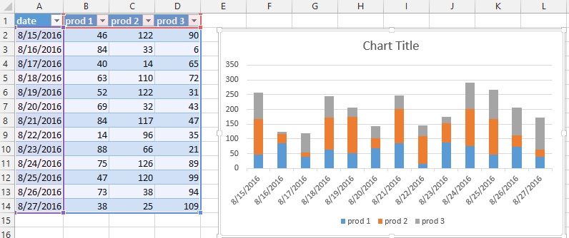 796×334 create dynamic chart excel from www.easyexcelanswers.com
 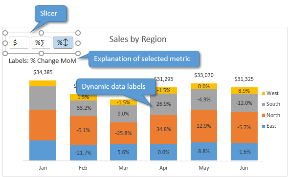 589×363 create dynamic chart data labels slicers excel campus from www.excelcampus.com
  694×410 create dynamic chart excel chart walls from chartwalls.blogspot.com
 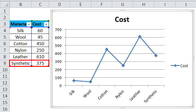 688×394 dynamic chart excel examples create dynamic chart excel from www.educba.com
  960×509 creating interactive charts slicers simply excel from simplyexcelcoza.weebly.com
  509×503 slicer controlled interactive excel charts from www.myonlinetraininghub.com
 How To Create Dynamic Charts In Excel With Slicers was posted in December 15, 2025 at 4:32 pm. If you wanna have it as yours, please click the Pictures and you will go to click right mouse then Save Image As and Click Save and download the How To Create Dynamic Charts In Excel With Slicers Picture.. Don’t forget to share this picture with others via Facebook, Twitter, Pinterest or other social medias! we do hope you'll get inspired by ExcelKayra... Thanks again! If you have any DMCA issues on this post, please contact us!