How To Create Dynamic Dependent Dropdown Lists In Excel
How To Create Dynamic Dependent Dropdown Lists In Excel - There are a lot of affordable templates out there, but it can be easy to feel like a lot of the best cost a amount of money, require best special design template. Making the best template format choice is way to your template success. And if at this time you are looking for information and ideas regarding the How To Create Dynamic Dependent Dropdown Lists In Excel then, you are in the perfect place. Get this How To Create Dynamic Dependent Dropdown Lists In Excel for free here. We hope this post How To Create Dynamic Dependent Dropdown Lists In Excel inspired you and help you what you are looking for.
“`html
Creating Dynamic Dependent Dropdown Lists in Excel
Dynamic dependent dropdown lists in Excel, also known as cascading dropdowns, allow you to create interactive spreadsheets where the options available in one dropdown list depend on the selection made in another. This enhances data entry accuracy and provides a more user-friendly experience. This guide will walk you through the process of creating these dynamic lists, explaining each step with clear examples.
Understanding the Concept
The core idea behind dependent dropdowns is that the first dropdown (the ‘parent’ dropdown) drives the content of the subsequent dropdowns (the ‘child’ dropdowns). For instance, you might have a parent dropdown for ‘Country’ and a child dropdown for ‘City.’ Selecting ‘USA’ in the Country dropdown will then display a list of US cities in the City dropdown.
Steps to Create Dynamic Dependent Dropdowns
-
Prepare Your Data
The foundation of your dynamic dropdowns is well-organized data. You’ll need a table or named ranges that define the relationship between your dropdown lists. Let’s use the ‘Country’ and ‘City’ example. Your data should look similar to this:
Country | City ------------|------------------- USA | New York USA | Los Angeles USA | Chicago Canada | Toronto Canada | Montreal Canada | Vancouver UK | London UK | Manchester UK | BirminghamEnsure your data is consistently formatted, and there are no typos or inconsistencies in the parent category values (e.g., ensure “USA” is always “USA,” not sometimes “U.S.A.” or “United States”).
-
Create Named Ranges for Parent Categories
Assign a name to the range containing the unique values from your *parent* dropdown. In our example, this is the ‘Country’ column.
- Select the entire ‘Country’ column (e.g., A2:A10, excluding the header).
- Go to the ‘Formulas’ tab in the Excel ribbon.
- Click on ‘Define Name’ (or use the shortcut Ctrl+Shift+F3, or Cmd+Shift+F3 on macOS).
- In the ‘Name’ field, type a descriptive name like “CountryList”. Avoid spaces in the name; use underscores instead if necessary (e.g., “Country_List”).
- Make sure the ‘Refers to’ field accurately reflects the selected range (e.g., ‘=Sheet1!$A$2:$A$10’).
- Click ‘OK’.
Next, create a *unique* list of countries for validation. To do this, select the column again and use “Data” > “Remove Duplicates” (found under the Data Tools section). This will leave you with a single instance of each country to create your initial dropdown.
-
Create Named Ranges for Child Categories (using INDIRECT)
This is the crucial step that establishes the dependency. You’ll create named ranges for each parent category, encompassing its corresponding child category values. We will use the
INDIRECTfunction here.- Select the data for the first country (e.g., for ‘USA’, select B2:B4).
- Go to the ‘Formulas’ tab and click ‘Define Name’.
- In the ‘Name’ field, type the exact name of the parent category (e.g., “USA”). This name must match the values in your ‘Country’ column perfectly.
- Ensure the ‘Refers to’ field is correct (e.g., ‘=Sheet1!$B$2:$B$4’).
- Click ‘OK’.
- Repeat this process for each country (‘Canada’, ‘UK’, etc.), selecting the corresponding city ranges and naming the ranges after the respective countries.
-
Create the Parent Dropdown
Now, create the first dropdown list for the ‘Country’.
- Select the cell where you want the ‘Country’ dropdown to appear (e.g., D2).
- Go to the ‘Data’ tab.
- Click on ‘Data Validation’.
- In the ‘Settings’ tab, under ‘Allow’, select ‘List’.
- In the ‘Source’ field, type `=CountryList` (the name you assigned to the list of unique countries).
- Click ‘OK’.
You should now have a dropdown list in cell D2 containing your list of countries.
-
Create the Dependent Child Dropdown (using INDIRECT)
This is where the magic happens! You’ll use the
INDIRECTfunction in the ‘Source’ field of the child dropdown’s data validation.- Select the cell where you want the ‘City’ dropdown to appear (e.g., E2).
- Go to the ‘Data’ tab.
- Click on ‘Data Validation’.
- In the ‘Settings’ tab, under ‘Allow’, select ‘List’.
- In the ‘Source’ field, type `=INDIRECT(D2)`. This tells Excel to use the value selected in cell D2 (the ‘Country’ selection) as the name of the range to use for the list.
- Click ‘OK’.
The
INDIRECTfunction uses the *text* inside cell D2 as a range name. Since you’ve named ranges “USA,” “Canada,” and “UK” (corresponding to the city lists),INDIRECTdynamically retrieves the correct city list based on the chosen country.
Important Considerations
- Naming Conventions: Consistency in naming ranges is crucial. Ensure the names you use for your named ranges exactly match the values in your parent dropdown. Any discrepancies will cause the dependent dropdowns to fail.
- Error Handling: If the parent dropdown cell is empty, the child dropdown will likely display an error. You can use conditional formatting or data validation messages to handle these scenarios gracefully, informing the user to select a country first.
- Data Structure: A well-organized data table is essential. While the above example is simple, you can extend this to multiple levels of dependencies (e.g., Country -> State -> City). However, the complexity of your data table will increase accordingly.
- Using Tables: Consider using Excel tables instead of simple ranges. Tables automatically adjust named ranges as you add or remove data, reducing the need to manually update them. You can reference table columns using structured references (e.g., `TableName[ColumnName]`).
Example with Tables
If your data is in a table named “LocationData” with columns “Country” and “City”, the named range definitions and data validation steps would change slightly:
- Create a “CountryList” using the UNIQUE() function. If the full “Country” column (including the header) were placed in cell G1, then create a named range “CountryList” with the definition `=UNIQUE(LocationData[Country])`
- For the ‘City’ named ranges, instead of referring to specific cell ranges, use: `=FILTER(LocationData[City],LocationData[Country]=H1)` where H1 represents the value in the “CountryList” column of the table. This can be entered in cell I1 and then dragged downwards for each country, then name each result with the corresponding country from column G.
- Use the named “CountryList” range as the source for your primary dropdown.
- Use `INDIRECT(D2)` as the source for your secondary dropdown as before.
By following these steps and carefully managing your data, you can create powerful and user-friendly dynamic dependent dropdown lists in Excel that streamline data entry and improve the overall quality of your spreadsheets.
“`
 512×292 excel dynamic dependent dropdown lists office bytes from itstraining.wichita.edu
 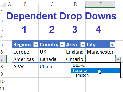 400×299 choose excel dependent drop setup method from www.contextures.com
  600×315 dependent drop lists excel step step tutorial from www.excel-easy.com
  521×362 create dependent drop lists excel campus from www.excelcampus.com
 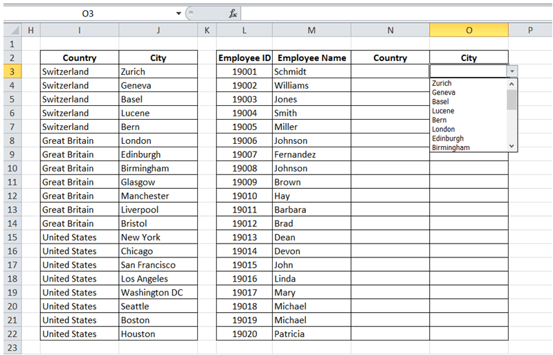 799×513 excelmadeeasy dependent drop lists excel from excelmadeeasy.com
  768×572 create dynamic drop list excel excel unlocked from excelunlocked.com
  755×681 create simple dynamicdependent drop lists excel ideas from merkez-ihayat.blogspot.com
  919×544 create dependent drop list excel gyankosh from gyankosh.net
  897×497 quickly create dynamic drop list excel from www.extendoffice.com
  908×438 create dependent drop list excel xl cad from xlncad.com
  951×248 create multiple dependent drop downs array formulas from www.p2w2.com
  864×480 create multi level dependent drop list excel from www.extendoffice.com
 How To Create Dynamic Dependent Dropdown Lists In Excel was posted in January 25, 2026 at 7:11 am. If you wanna have it as yours, please click the Pictures and you will go to click right mouse then Save Image As and Click Save and download the How To Create Dynamic Dependent Dropdown Lists In Excel Picture.. Don’t forget to share this picture with others via Facebook, Twitter, Pinterest or other social medias! we do hope you'll get inspired by ExcelKayra... Thanks again! If you have any DMCA issues on this post, please contact us!