How To Create KPI Dashboard In Excel For Small Business
How To Create KPI Dashboard In Excel For Small Business - There are a lot of affordable templates out there, but it can be easy to feel like a lot of the best cost a amount of money, require best special design template. Making the best template format choice is way to your template success. And if at this time you are looking for information and ideas regarding the How To Create KPI Dashboard In Excel For Small Business then, you are in the perfect place. Get this How To Create KPI Dashboard In Excel For Small Business for free here. We hope this post How To Create KPI Dashboard In Excel For Small Business inspired you and help you what you are looking for.
Creating a KPI (Key Performance Indicator) dashboard in Excel for a small business allows you to visually track and monitor your business performance, identify trends, and make data-driven decisions. A well-designed dashboard provides a clear and concise overview of your most important metrics, helping you stay on track towards your goals.
1. Define Your KPIs
The first and most crucial step is identifying the KPIs relevant to your business. These should align with your overall strategic objectives. Ask yourself:
- What are the most critical aspects of my business I need to monitor?
- What metrics directly impact my profitability, growth, and customer satisfaction?
- What are my key goals, and how can I measure progress towards them?
Examples of KPIs for small businesses might include:
- Sales Revenue: Total revenue generated from sales.
- Customer Acquisition Cost (CAC): The cost of acquiring a new customer.
- Customer Lifetime Value (CLTV): The predicted revenue a customer will generate during their relationship with your business.
- Gross Profit Margin: The percentage of revenue remaining after deducting the cost of goods sold.
- Website Traffic: The number of visitors to your website.
- Conversion Rate: The percentage of website visitors who complete a desired action (e.g., making a purchase, filling out a form).
- Customer Satisfaction Score (CSAT): A measure of customer satisfaction with your products or services.
- Employee Turnover Rate: The rate at which employees leave your company.
- Inventory Turnover Rate: The rate at which inventory is sold and replaced.
- Social Media Engagement: Metrics like likes, shares, comments, and follows on social media platforms.
Choose a manageable number of KPIs, typically between 5 and 10, to avoid overwhelming your dashboard. Ensure your KPIs are SMART: Specific, Measurable, Achievable, Relevant, and Time-bound.
2. Collect and Organize Your Data
Once you’ve identified your KPIs, you need to gather the data required to calculate them. This data may come from various sources, such as:
- Sales records
- Accounting software
- CRM systems
- Website analytics platforms (e.g., Google Analytics)
- Social media analytics tools
- Customer surveys
Organize your data in a structured format within Excel. Create separate sheets for each data source or category. Ensure your data is consistent and accurate. Use clear column headers and consistent data formats (e.g., dates, numbers, currencies).
Consider using Excel Tables to store your data. Tables automatically expand as you add new data and allow you to use structured references in formulas, making your calculations more robust and easier to understand.
3. Calculate Your KPIs
Using the data you’ve collected, calculate your KPIs using Excel formulas. For example, if you’re tracking sales revenue, you might use the `SUM` function to calculate the total sales for a given period. For more complex KPIs, you may need to use more advanced formulas or functions like `AVERAGE`, `IF`, `VLOOKUP`, or `SUMIFS`.
Create a dedicated sheet for your KPI calculations. This keeps your raw data separate from your calculated metrics, making it easier to maintain and update your dashboard. Clearly label each KPI and the corresponding formula used to calculate it.
4. Design Your Dashboard
Now that you have your KPIs calculated, it’s time to create the visual dashboard. Here’s how:
- Create a new sheet: Name it “Dashboard” or something similar.
- Choose appropriate visualizations: Select chart types that best represent your data. Common options include:
- Line charts: To show trends over time.
- Column/Bar charts: To compare values across different categories.
- Pie charts: To show proportions of a whole (use sparingly, as they can be difficult to read).
- Gauge charts: To show progress towards a target. (Requires installing a add-in, might not be suitable for all excel versions)
- Number cards: To display key values prominently.
- Add charts and visualizations: Insert your chosen charts and link them to the KPI calculations on your KPI calculations sheet. To do this, select the chart, go to “Design” tab, then “Select Data.” In the “Chart data range” field, select the range containing your KPI data.
- Use clear labels and titles: Ensure each chart and KPI is clearly labeled with descriptive titles and axis labels. This makes it easy for viewers to understand the information being presented.
- Use color effectively: Use color strategically to highlight key information and draw attention to important trends. Avoid using too many colors, as this can be distracting. Consider using a consistent color scheme across your dashboard.
- Add filters and slicers: Allow users to filter the data by date range, region, product category, or other relevant criteria. Slicers provide a visual way to filter data. To add slicers, select a cell within a table containing your data, go to the “Insert” tab, and click “Slicer.”
- Arrange elements logically: Organize the dashboard elements in a logical and intuitive way. Place the most important KPIs at the top and center of the dashboard. Group related KPIs together.
5. Add Conditional Formatting
Conditional formatting can help you quickly identify areas that need attention. For example, you could use conditional formatting to:
- Highlight KPIs that are below target.
- Color-code data based on performance (e.g., green for good, yellow for average, red for poor).
- Create data bars to visually represent the magnitude of values.
To add conditional formatting, select the range of cells you want to format, go to the “Home” tab, and click “Conditional Formatting.” Choose a rule that suits your needs.
6. Automate Updates
To ensure your dashboard is always up-to-date, automate the data import and calculation process as much as possible. This can be done using:
- Excel Power Query: To import and transform data from various sources.
- Excel Macros (VBA): To automate repetitive tasks.
- Data connections: If your data resides in a database, connect directly to the database using Excel’s data connection features.
By automating the update process, you can save time and ensure your dashboard always reflects the most current information.
7. Regularly Review and Refine
Your KPI dashboard is not a static document. Regularly review it to ensure it’s still relevant and effective. As your business evolves, your KPIs may need to change. Gather feedback from users to identify areas for improvement. Experiment with different visualizations and layouts to find what works best for your team.
By following these steps, you can create a powerful KPI dashboard in Excel that helps you track your business performance, identify trends, and make informed decisions.
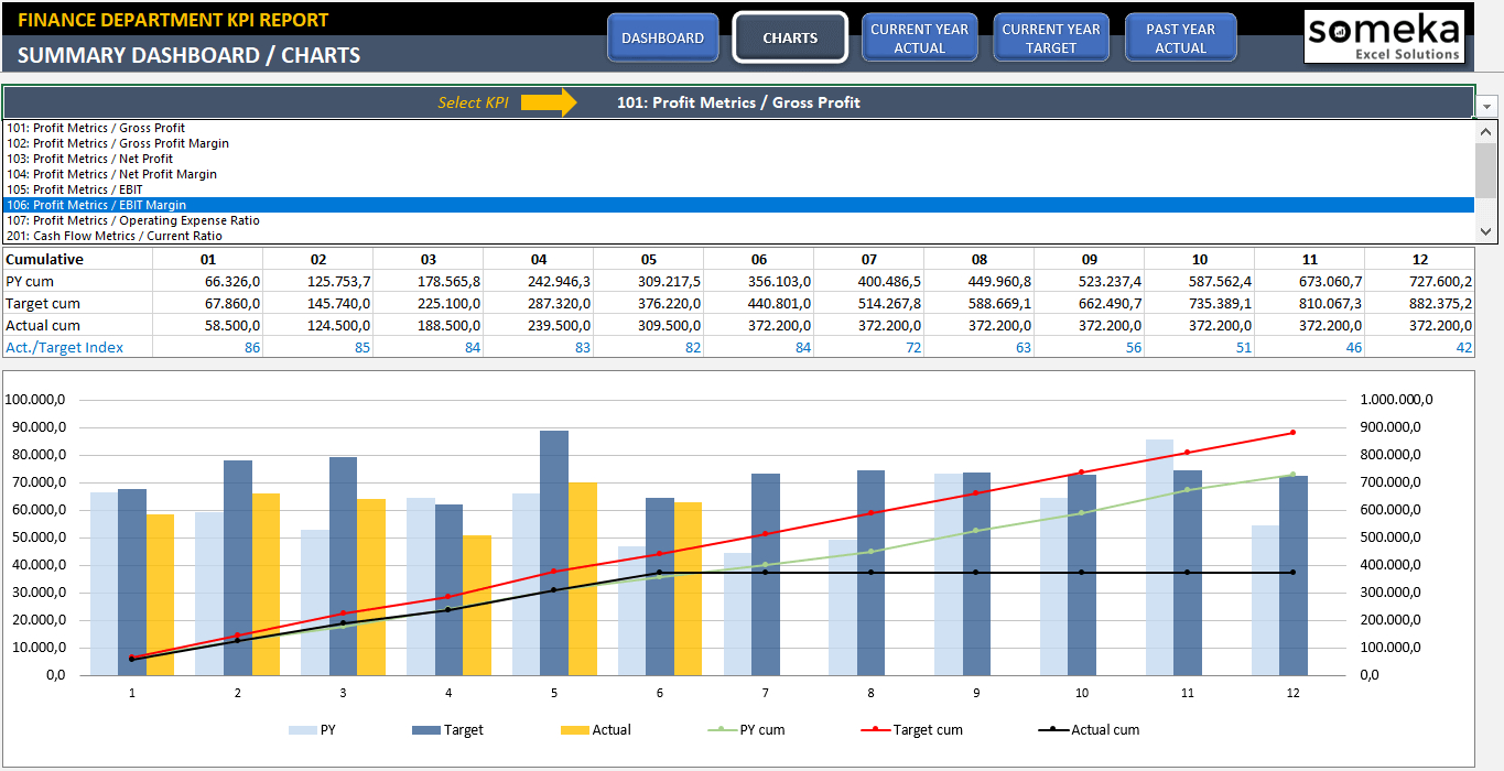 1365×700 business kpi dashboard excel db excelcom from db-excel.com
  1200×675 business kpi dashboard excel business spreadshee business kpi dashboard from db-excel.com
  1280×720 management kpi dashboard ready professional excel template from www.someka.net
  1365×700 management kpi dashboard excel template kpis general managers from www.someka.net
  1400×889 kpi dashboards comprehensive guide examples simplekpi from db-excel.com
  1024×493 flying blind focused kpi dashboard from cfoperspective.com
  1365×700 kpi dashboard excel template db excelcom from db-excel.com
  1169×642 making simple kpi dashboard ms excel from chandoo.org
  706×443 create simple kpi dashboard excel rachel pemelton medium from medium.com
 How To Create KPI Dashboard In Excel For Small Business was posted in July 11, 2025 at 1:44 pm. If you wanna have it as yours, please click the Pictures and you will go to click right mouse then Save Image As and Click Save and download the How To Create KPI Dashboard In Excel For Small Business Picture.. Don’t forget to share this picture with others via Facebook, Twitter, Pinterest or other social medias! we do hope you'll get inspired by ExcelKayra... Thanks again! If you have any DMCA issues on this post, please contact us!