How To Transpose Data In Excel Without Paste Special
How To Transpose Data In Excel Without Paste Special - There are a lot of affordable templates out there, but it can be easy to feel like a lot of the best cost a amount of money, require best special design template. Making the best template format choice is way to your template success. And if at this time you are looking for information and ideas regarding the How To Transpose Data In Excel Without Paste Special then, you are in the perfect place. Get this How To Transpose Data In Excel Without Paste Special for free here. We hope this post How To Transpose Data In Excel Without Paste Special inspired you and help you what you are looking for.
“`html
Transposing Data in Excel Without Paste Special
Transposing data in Excel—that is, swapping rows and columns—is a common task, but the traditional method involving “Paste Special” with the “Transpose” option can be cumbersome, especially when dealing with dynamic data that needs to update automatically. Fortunately, Excel offers several alternative methods to achieve transposition without relying on Paste Special, each with its own strengths and suitable use cases. This article explores these techniques, empowering you to choose the most efficient approach for your specific needs.
Understanding the Need for Alternative Transposition Methods
While Paste Special is a straightforward way to transpose static data, it creates a static copy. Any changes to the original data range won’t be reflected in the transposed version. This limitation necessitates exploring dynamic alternatives that automatically update the transposed data when the source data changes. These dynamic approaches are particularly valuable in scenarios where you are working with live data feeds, regularly updated tables, or interactive dashboards.
Method 1: Using the TRANSPOSE Function
The TRANSPOSE function is the most direct and versatile method for dynamic transposition. It’s an array function, meaning it operates on a range of cells and returns a range of cells. Here’s how to use it:
- Select the Target Range: Determine the dimensions of your original data. If your original data is, say, 5 rows and 3 columns, you’ll need to select a range that is 3 rows and 5 columns to accommodate the transposed data. It’s crucial to select the correct number of cells beforehand.
- Enter the Formula: With the target range selected, type
=TRANSPOSE(in the formula bar. - Specify the Source Range: Select the range of cells containing the data you want to transpose, or manually type the cell range (e.g.,
A1:C5). - Close the Parenthesis: Add a closing parenthesis to complete the formula:
=TRANSPOSE(A1:C5). - Enter as an Array Formula: This is the crucial step. Instead of pressing Enter, press Ctrl + Shift + Enter (Command + Shift + Enter on a Mac). This tells Excel to treat the formula as an array formula and populate the entire selected range with the transposed values.
Important Considerations for the TRANSPOSE Function:
- Array Formula Confirmation: Excel will automatically enclose the formula in curly braces
{}. Do not type these braces manually; Excel adds them to indicate an array formula. If you try to edit a single cell within the transposed range, you’ll likely encounter an error because you’re attempting to modify part of an array. To modify the transposed data, you must change the original data range or re-enter the entireTRANSPOSEformula after selecting the whole output range. - Deleting Data: You cannot delete individual cells within the transposed range. You must delete the entire array formula output by selecting the entire output range and pressing Delete.
- Dynamic Updates: The
TRANSPOSEfunction is dynamic. Any changes made to the original data range will automatically update the transposed data. - Blank Cells: The
TRANSPOSEfunction handles blank cells gracefully; they will simply be transposed as blank cells.
Method 2: Using INDEX and ROW/COLUMN Functions
This method leverages the INDEX, ROW, and COLUMN functions to dynamically transpose data. It’s slightly more complex than the TRANSPOSE function but offers greater flexibility in some scenarios.
- Identify the Starting Cell: Choose a cell where you want the transposed data to begin.
- Enter the Formula: In that cell, enter the following formula (adjusting the cell ranges accordingly):
=INDEX(OriginalDataRange,COLUMN(A1),ROW(A1))ReplaceOriginalDataRangewith the actual cell range of your original data (e.g.,$A$1:$C$5). Note the use of absolute references ($) for the original data range to prevent it from shifting when copying the formula.A1is used as a reference point and will adjust as the formula is copied; you can use any cell here, but `A1` is conventional. - Copy the Formula: Copy the formula across and down to cover the transposed dimensions of your data. If your original data is 5 rows and 3 columns, copy the formula 3 rows and 5 columns.
Explanation of the Formula:
- INDEX Function: The
INDEXfunction returns the value of a cell within a given range based on its row and column number. - ROW(A1): The
ROW(A1)function returns the row number of cell A1, which is 1. As you copy the formula down,ROW(A1)will becomeROW(A2),ROW(A3), and so on, effectively generating the row numbers 1, 2, 3, etc. - COLUMN(A1): The
COLUMN(A1)function returns the column number of cell A1, which is 1. As you copy the formula across,COLUMN(A1)will becomeCOLUMN(B1),COLUMN(C1), and so on, effectively generating the column numbers 1, 2, 3, etc. - How it Transposes: By swapping the row and column arguments within the
INDEXfunction with theROWandCOLUMNfunctions, we effectively transpose the data. The row numbers from the transposed location drive the column selection from the original data, and the column numbers from the transposed location drive the row selection from the original data.
Advantages of Using INDEX and ROW/COLUMN:
- Dynamic Updates: Like the
TRANSPOSEfunction, this method dynamically updates the transposed data when the original data changes. - Flexibility: This method offers greater flexibility in terms of where you place the transposed data and how you structure it. You can insert columns or rows within the transposed range without disrupting the formula’s functionality (as long as you adjust the formula if necessary).
- Handling Blank Cells: Similar to the
TRANSPOSEfunction, blank cells are handled correctly.
Method 3: Power Query (Get & Transform Data)
Power Query, available in recent versions of Excel (Excel 2010 and later as an add-in, built-in from Excel 2016), provides a powerful and flexible way to transform data, including transposing it. This method is particularly useful when dealing with data from external sources or when you need to perform more complex data cleaning and transformation operations in addition to transposition.
- Load Data into Power Query: Select your data range in Excel. Go to the “Data” tab and click “From Table/Range”. This will open the Power Query Editor.
- Transpose the Data: In the Power Query Editor, select your data. Go to the “Transform” tab and click “Transpose”.
- Close & Load: Click “Close & Load” (or “Close & Load To…”) to load the transposed data back into your Excel worksheet. You can choose to load it into a new worksheet or an existing one.
Advantages of Using Power Query:
- Powerful Data Transformation: Power Query offers a wide range of data transformation capabilities beyond just transposition, including filtering, sorting, grouping, merging, and data cleaning.
- Connection to External Data Sources: Power Query can connect to various data sources, such as databases, web pages, and text files, making it ideal for transposing data from external sources.
- Refreshable Queries: Power Query queries can be refreshed, meaning that if the underlying data changes, you can easily update the transposed data with a simple click.
- Step-by-Step Transformation: The Power Query editor records each step of your transformation. This makes it easier to understand, modify and repeat your transformation process.
Choosing the Right Method
The best method for transposing data without Paste Special depends on your specific needs and circumstances:
TRANSPOSEFunction: Use this when you need a simple and direct dynamic transposition within your Excel worksheet. It is the quickest method if you only need to transpose.INDEXandROW/COLUMNFunctions: Choose this method when you need more flexibility in terms of data placement and structure within your worksheet.- Power Query: Use Power Query when you are dealing with data from external sources, need to perform more complex data transformations beyond transposition, or require refreshable queries.
By mastering these alternative transposition methods, you can enhance your efficiency and create more dynamic and interactive Excel workbooks.
“`
 414×346 easy ways transpose data excel quickexcel from quickexcel.com
  395×276 transpose data excel step step guide from trumpexcel.com
  866×522 day transpose excel data paste special tracy van der schyff from tracyvanderschyff.com
  675×300 transpose columns rows paste special excel laptop mag from www.laptopmag.com
  355×214 excel paste transpose transpose function paste special from www.wallstreetmojo.com
  629×399 transpose columns rows paste data excel from www.extendoffice.com
  1738×715 transpose excel columns rows paste special from yodalearning.com
  1241×705 step cut paste transpose excel from www.howtoexcel.org
 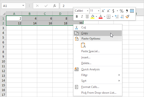 604×407 transpose data excel step step tutorial from www.excel-easy.com
  970×723 excel paste link paste special transpose data excel work from www.excelatwork.co.nz
 How To Transpose Data In Excel Without Paste Special was posted in October 17, 2025 at 2:15 am. If you wanna have it as yours, please click the Pictures and you will go to click right mouse then Save Image As and Click Save and download the How To Transpose Data In Excel Without Paste Special Picture.. Don’t forget to share this picture with others via Facebook, Twitter, Pinterest or other social medias! we do hope you'll get inspired by ExcelKayra... Thanks again! If you have any DMCA issues on this post, please contact us!