How To Split Text Into Columns In Excel Using Formulas
How To Split Text Into Columns In Excel Using Formulas - There are a lot of affordable templates out there, but it can be easy to feel like a lot of the best cost a amount of money, require best special design template. Making the best template format choice is way to your template success. And if at this time you are looking for information and ideas regarding the How To Split Text Into Columns In Excel Using Formulas then, you are in the perfect place. Get this How To Split Text Into Columns In Excel Using Formulas for free here. We hope this post How To Split Text Into Columns In Excel Using Formulas inspired you and help you what you are looking for.
Splitting Text into Columns in Excel Using Formulas
Excel’s “Text to Columns” feature is a powerful tool for quickly dividing data. However, for more dynamic and automated workflows, formulas offer greater flexibility. This guide explores various Excel formulas that enable you to split text strings into separate columns, adapting to different delimiters, positions, and complexities.
Basic Splitting Using LEFT, RIGHT, and MID
The fundamental formulas for text manipulation are LEFT, RIGHT, and MID. These, combined with FIND or SEARCH, can extract portions of a text string based on the position of a delimiter.
LEFT(text, num_chars): Returns the specified number of characters from the *beginning* of a text string.RIGHT(text, num_chars): Returns the specified number of characters from the *end* of a text string.MID(text, start_num, num_chars): Returns a specific number of characters from a text string, starting at the position you specify.FIND(find_text, within_text, [start_num]): Returns the starting position of one text string within another. Case-sensitive.SEARCH(find_text, within_text, [start_num]): Returns the starting position of one text string within another. Not case-sensitive and allows wildcard characters.
Splitting by a Single, Consistent Delimiter
Suppose you have data in column A, such as “John,Doe,30”, where the delimiter is a comma (,). To split this into three columns (First Name, Last Name, Age), use the following formulas:
In cell B1 (First Name):
=LEFT(A1,FIND(",",A1)-1)Explanation: This extracts characters from the left side of A1 up to the character *before* the first comma. FIND(",",A1) locates the position of the comma, and subtracting 1 ensures that the comma itself isn’t included in the result.
In cell C1 (Last Name):
=MID(A1,FIND(",",A1)+1,FIND(",",A1,FIND(",",A1)+1)-FIND(",",A1)-1)Explanation: This is more complex. It extracts characters starting *after* the first comma. FIND(",",A1)+1 determines the starting position. FIND(",",A1,FIND(",",A1)+1) finds the *second* comma. Subtracting FIND(",",A1) and 1 determines the number of characters to extract – the length between the first and second commas.
In cell D1 (Age):
=RIGHT(A1,LEN(A1)-FIND(",",A1,FIND(",",A1)+1))Explanation: This extracts the characters from the right side of A1. LEN(A1) gives the total length of the string. Subtracting the position of the second comma (FIND(",",A1,FIND(",",A1)+1)) gives the number of characters to extract from the right.
Drag these formulas down to apply them to the rest of your data in column A.
Handling Varying Numbers of Delimiters
The above formulas work when the number of delimiters is consistent. If you have a varying number, you’ll need to adapt the formulas. A common approach is to use the IFERROR function to handle cases where a delimiter is missing.
For example, if some entries in column A only have “John,Doe” (missing the age), the previous formulas will return an error for the “Age” column. To prevent this, use:
In cell D1 (Age, handling missing values):
=IFERROR(RIGHT(A1,LEN(A1)-FIND(",",A1,FIND(",",A1)+1)),"")Explanation: IFERROR catches any errors produced by the original RIGHT formula. If an error occurs (because the second comma isn’t found), it returns an empty string (“”), effectively leaving the “Age” cell blank.
Advanced Splitting with TEXTSPLIT (Excel 365 and later)
Excel 365 introduced the TEXTSPLIT function, significantly simplifying text splitting tasks.
TEXTSPLIT(text, col_delimiter, [row_delimiter], [ignore_empty], [match_mode], [pad_with]): Splits text into columns and/or rows using specified delimiters.
Splitting with TEXTSPLIT
Using the same “John,Doe,30” example, the formula becomes much simpler:
In cell B1 (First Name, Last Name, Age):
=TEXTSPLIT(A1,",")Explanation: This single formula splits the text in A1 using the comma (,) as a column delimiter. The results will automatically spill into the adjacent columns (B1, C1, D1) if those cells are empty. If the adjacent cells contain data, a #SPILL! error will be shown.
Handling Multiple Delimiters and Empty Values with TEXTSPLIT
TEXTSPLIT can also handle multiple delimiters. For example, if the data in A1 is “John,Doe;30”, you can split by both comma and semicolon:
=TEXTSPLIT(A1,{",",";"})The {",",";"} is an array constant, specifying multiple delimiters. The ignore_empty argument can be set to TRUE to skip empty values if delimiters appear consecutively.
Splitting by Character Position
Sometimes, you need to split text based on character position rather than delimiters. LEFT, RIGHT, and MID are suitable for this.
For example, if column A contains serial numbers formatted as “ABC12345”, where the first three characters are a code and the remaining five are a number:
In cell B1 (Code):
=LEFT(A1,3)In cell C1 (Number):
=RIGHT(A1,5)Considerations and Best Practices
- Error Handling: Always use
IFERRORto handle potential errors arising from missing delimiters or unexpected data formats. - Data Consistency: Ensure your data is as consistent as possible. Inconsistent delimiters or formats will require more complex formulas.
- Alternatives: For complex splitting scenarios, consider using Power Query (Get & Transform Data), which offers more advanced data cleaning and transformation capabilities without relying solely on formulas.
- Performance: While formulas offer flexibility, using too many complex formulas can slow down your spreadsheet. For large datasets, Power Query may be more efficient.
- TEXTJOIN: The
TEXTJOINfunction (available in Excel 365 and later) is the inverse ofTEXTSPLITand allows you to combine text strings with a delimiter. This is useful for putting split data back together in a different format.
Example: Splitting Full Names
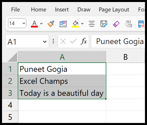
A common task is splitting a full name (“John Doe”) into first and last names. This is complicated by middle names or initials. Here’s a formula using TEXTBEFORE and TEXTAFTER (Excel 365 and later) that handles some of these cases:
In cell B1 (First Name):
=TEXTBEFORE(A1," ")In cell C1 (Last Name):
=TEXTAFTER(A1," ",-1)Explanation: TEXTBEFORE gets the text *before* the first space. TEXTAFTER gets the text *after* the *last* space (the -1 specifies the last occurrence). This correctly extracts the last name even if there are middle names or initials. It is important to note that this only works in Excel 365.
While not perfect (it won’t handle names with titles or suffixes perfectly), this provides a good starting point and is more robust than simpler formulas.
Conclusion
Excel formulas provide a powerful way to split text into columns. Understanding the functions LEFT, RIGHT, MID, FIND, SEARCH, and TEXTSPLIT (if available) allows you to handle a wide range of text splitting scenarios. Always consider error handling, data consistency, and performance when choosing the best approach for your specific needs.
 513×437 split text space excel formula from excelchamps.com
  700×400 split text delimiter excel formula exceljet from exceljet.net
  1632×1029 split text columns excel formula templates from campolden.org
  656×386 split text columns excel formula printable from printableformsfree.com
  810×711 split text multiple columns text column excel from campolden.org
  700×400 excel formula split text string specific character exceljet from exceljet.net
  696×464 split text columns formula excel dynamic array from infoinspired.com
  1867×559 split texts cells text columns fix excel errors from fixallexcelerrors.com
  400×400 split text excel columns functions excel from cz.pinterest.com
 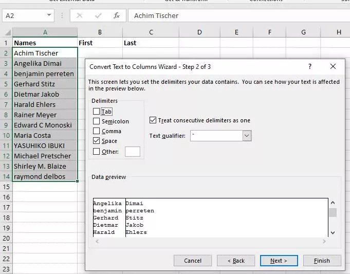 474×370 split text columns excel pcauthoritiescom from pcauthorities.com
  683×671 split text columns excel healthy food from healthy-food-near-me.com
  1280×720 excel text column split text multiple columns aspose hot from www.hotzxgirl.com
 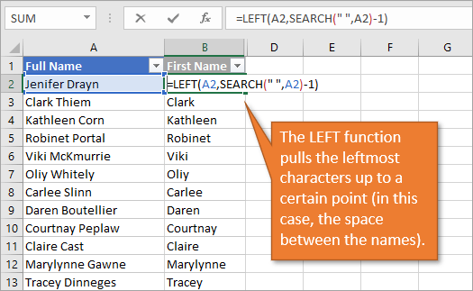 525×323 split text cells formulas excel campus from www.excelcampus.com
  655×408 split complicated text columns microsoft community hub from techcommunity.microsoft.com
 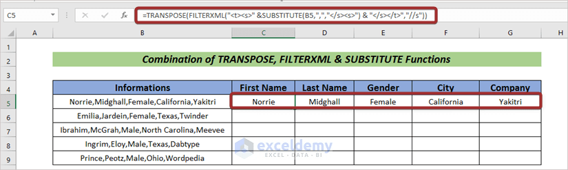 825×247 split text columns automatically formula excel ways from www.exceldemy.com
  440×335 split text columns excel specific column contextures blog from contexturesblog.com
 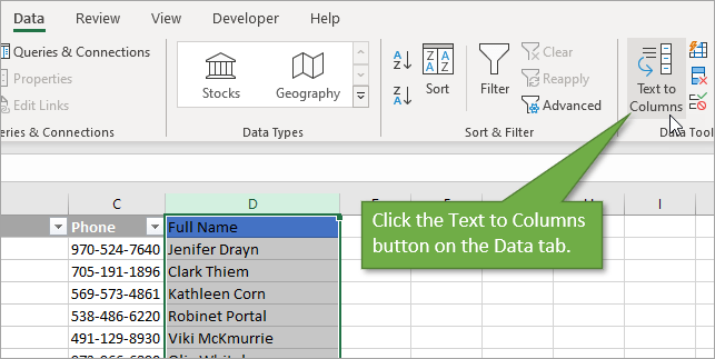 643×323 split cells text columns excel excel campus from www.excelcampus.com
 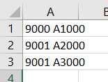 155×118 excel basics separate text columns learn excel from www.learnexcelnow.com
  880×477 excel text columns split data multiple columns from www.powerusersoftwares.com
 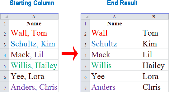 543×307 split text data columns keynote support from www.keynotesupport.com
  1920×1080 excel text columns split data multiple columns www from www.vrogue.co
 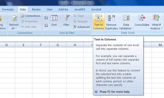 538×323 split text data cell column excel exceldatapro from exceldatapro.com
 How To Split Text Into Columns In Excel Using Formulas was posted in October 22, 2025 at 8:02 am. If you wanna have it as yours, please click the Pictures and you will go to click right mouse then Save Image As and Click Save and download the How To Split Text Into Columns In Excel Using Formulas Picture.. Don’t forget to share this picture with others via Facebook, Twitter, Pinterest or other social medias! we do hope you'll get inspired by ExcelKayra... Thanks again! If you have any DMCA issues on this post, please contact us!