Home » Excel Templates » How To Use Conditional Formatting To Highlight Overdue Tasks In Excel

How To Use Conditional Formatting To Highlight Overdue Tasks In Excel

Thursday, January 8th 2026. | Excel Templates

How To Use Conditional Formatting To Highlight Overdue Tasks In Excel - There are a lot of affordable templates out there, but it can be easy to feel like a lot of the best cost a amount of money, require best special design template. Making the best template format choice is way to your template success. And if at this time you are looking for information and ideas regarding the How To Use Conditional Formatting To Highlight Overdue Tasks In Excel then, you are in the perfect place. Get this How To Use Conditional Formatting To Highlight Overdue Tasks In Excel for free here. We hope this post How To Use Conditional Formatting To Highlight Overdue Tasks In Excel inspired you and help you what you are looking for.

formula friday highlight overdue tasks conditional formatting

Highlighting Overdue Tasks with Conditional Formatting in Excel

Keeping track of deadlines is crucial for effective project management and personal productivity. Excel’s conditional formatting feature provides a powerful and dynamic way to visually highlight overdue tasks, ensuring they don’t slip through the cracks. This guide will walk you through the steps of using conditional formatting to highlight overdue tasks in Excel, covering various scenarios and customization options.

Understanding the Basics

Conditional formatting allows you to automatically apply formatting (e.g., background color, font style, icons) to cells based on specific criteria. For highlighting overdue tasks, we’ll use formulas that compare task due dates with the current date.

Setting Up Your Task List

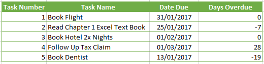
First, let’s assume you have an Excel sheet with the following columns:

Task Name: (Column A) The name or description of the task.
Due Date: (Column B) The date the task is due. This column should be formatted as a date.
Status: (Column C) (Optional) Indicates the current status of the task (e.g., “In Progress”, “Completed”, “Pending”). This column can be used for more refined conditional formatting.

Populate the sheet with your tasks, their due dates, and optionally their current status. Ensure that the Due Date column contains valid date entries that Excel recognizes.

Applying Conditional Formatting to Highlight Overdue Tasks

Here’s how to highlight overdue tasks based solely on the due date:

Select the Range: Select the range of cells containing the due dates (e.g., B2:B100). This is the range to which the conditional formatting will be applied.
Open Conditional Formatting: Go to the “Home” tab on the Excel ribbon. In the “Styles” group, click “Conditional Formatting.”
Create a New Rule: From the dropdown menu, select “New Rule…”
Choose Rule Type: In the “New Formatting Rule” dialog box, select “Use a formula to determine which cells to format.”
Enter the Formula: In the “Format values where this formula is true” box, enter the following formula:
=B2<TODAY()
Explanation:
- B2: Refers to the first cell in the selected range (the first due date). This is important because the formula will be applied relatively to the other cells in the range.
- <: Is the “less than” operator, meaning “before”.
- TODAY(): Is an Excel function that returns the current date.
The formula checks if the due date in cell B2 is earlier than the current date. If it is, the condition is true, and the formatting will be applied.
Set the Formatting: Click the “Format…” button. This opens the “Format Cells” dialog box.
Choose Formatting Options: In the “Format Cells” dialog box, you can choose various formatting options such as:
- Fill: Set the background color to highlight overdue tasks (e.g., red or orange).
- Font: Change the font color (e.g., white or bold) to improve visibility.
- Border: Add a border to the cell.
Select your desired formatting and click “OK.”
Apply the Rule: Back in the “New Formatting Rule” dialog box, you’ll see a preview of the formatting you selected. Click “OK” to apply the rule.

Now, any task with a due date earlier than today’s date will be highlighted with the formatting you chose.

Highlighting Only Incomplete Overdue Tasks

If you have a “Status” column (Column C) indicating the completion status of the task, you can refine the conditional formatting to highlight only overdue tasks that are *not* completed.

Select the Range: Select the range of cells containing the due dates (e.g., B2:B100).
Open Conditional Formatting: Go to “Home” -> “Conditional Formatting” -> “New Rule…”
Choose Rule Type: Select “Use a formula to determine which cells to format.”
Enter the Formula: In the “Format values where this formula is true” box, enter a formula similar to this (adjust the “Status” values to match your sheet):
=AND(B2<TODAY(),C2<>"Completed")
Explanation:
- AND(): This function requires both conditions inside it to be true for the entire formula to be true.
- B2<TODAY(): Checks if the due date is earlier than today (same as before).
- C2<>"Completed": Checks if the status in column C is *not* equal to “Completed”. The <> operator means “not equal to”. You should replace “Completed” with whatever text you use to indicate a completed task. This part of the formula is case-sensitive if you are using text comparisons. You can use the UPPER() or LOWER() functions to make it case-insensitive, e.g., UPPER(C2)<>"COMPLETED"
This formula will only apply formatting if the due date is in the past *and* the status is not “Completed”.
Set the Formatting: Click the “Format…” button and choose your desired formatting options.
Apply the Rule: Click “OK” to apply the rule.

Now, only overdue tasks that are not marked as “Completed” (or your equivalent status) will be highlighted.

Highlighting the Entire Row

Instead of just highlighting the due date cell, you might want to highlight the entire row to make the overdue tasks more prominent. To do this, you need to adjust the formula slightly.

Select the Range: Select the *entire* range of cells containing the tasks you want to format, including the Task Name, Due Date, and Status columns (e.g., A2:C100). It is crucial to select the entire range that needs to be highlighted.
Open Conditional Formatting: Go to “Home” -> “Conditional Formatting” -> “New Rule…”
Choose Rule Type: Select “Use a formula to determine which cells to format.”
Enter the Formula: Use the same formulas as before, but with a crucial modification: use the $ sign to create an absolute reference to the *column* containing the Due Date (and Status, if applicable). For example:
- To highlight all overdue rows: =$B2<TODAY()
- To highlight only incomplete overdue rows: =AND($B2<TODAY(), $C2<>"Completed")
Explanation:
- The $ sign before the column letter (e.g., $B2) creates an absolute reference to the *column*. This means that as the conditional formatting is applied to other rows, the formula will always refer to column B (the Due Date column) for comparison. The row number (2) remains relative so that the formula correctly checks each row’s date.
Set the Formatting: Click the “Format…” button and choose your desired formatting options. This formatting will now be applied to the *entire row* when the condition is met.
Apply the Rule: Click “OK” to apply the rule.

Now, the entire row of an overdue task (or an incomplete overdue task) will be highlighted.

Managing Conditional Formatting Rules

You can manage and modify existing conditional formatting rules using the “Conditional Formatting Rules Manager”:

Go to “Home” -> “Conditional Formatting” -> “Manage Rules…”
In the “Conditional Formatting Rules Manager” dialog box, select the current worksheet or “This Worksheet” to see the rules applied to the current sheet.
You can then:
- Edit a Rule: Select a rule and click “Edit Rule…” to modify the formula or formatting.
- Delete a Rule: Select a rule and click “Delete Rule.”
- Adjust Rule Order: Use the “Move Up” and “Move Down” buttons to change the order in which the rules are applied. The order is important if you have multiple rules that might overlap.
- Change the Applied Range: Edit the “Applies to” field to change the range of cells to which the selected rule is applied.

Advanced Customization

Highlighting Tasks Due in the Next Week: You can modify the formula to highlight tasks due within a certain timeframe (e.g., the next week). Use a formula like =AND(B2>=TODAY(),B2<TODAY()+7) to highlight tasks due in the next 7 days.
Using Different Formatting for Different Levels of Overdue: You can create multiple conditional formatting rules with different formulas to highlight tasks that are overdue by different amounts of time (e.g., overdue by 1-7 days in yellow, overdue by more than 7 days in red). Remember that rule order is important.
Using Icons: Instead of background colors, you can use icon sets to visually represent the status of tasks (e.g., a red flag for overdue tasks, a yellow exclamation point for tasks due soon, a green checkmark for completed tasks). Explore the “Icon Sets” option under Conditional Formatting.
Named Ranges: Using named ranges can make your formulas more readable and easier to maintain. Instead of referring to “B2”, you can name the “Due Date” column (excluding the header) as “DueDate” and then use “DueDate” in your formula.

Conclusion

Conditional formatting is an invaluable tool for managing tasks and deadlines in Excel. By using formulas that compare due dates with the current date and incorporating status information, you can create a dynamic and visually informative task list that helps you stay organized and prioritize your work effectively. Experiment with different formatting options and formulas to tailor the conditional formatting to your specific needs and preferences.

520×128 formula friday highlight overdue tasks conditional formatting from howtoexcelatexcel.com

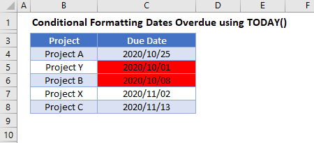450×205 conditional formatting overdue excel google sheets automate from www.automateexcel.com

706×442 conditional formatting highlight overdue solved excel from ccm.net

966×722 conditional formatting microsoft excel highlight information from xlinexcel.com

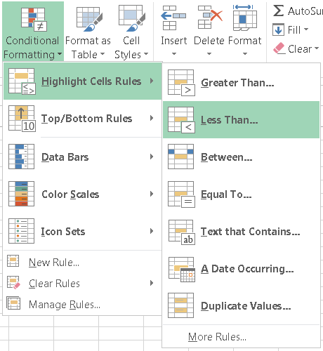460×500 conditional formatting highlight due excel learn from fiveminutelessons.com

900×526 guide conditional formatting excel from www.groovypost.com

471×133 conditional formatting excel from www.vertex42.com

How To Use Conditional Formatting To Highlight Overdue Tasks In Excel was posted in January 8, 2026 at 12:10 am. If you wanna have it as yours, please click the Pictures and you will go to click right mouse then Save Image As and Click Save and download the How To Use Conditional Formatting To Highlight Overdue Tasks In Excel Picture.. Don’t forget to share this picture with others via Facebook, Twitter, Pinterest or other social medias! we do hope you'll get inspired by ExcelKayra... Thanks again! If you have any DMCA issues on this post, please contact us!