Home » Excel Templates » How To Use The Offset Function In Excel With Examples

How To Use The Offset Function In Excel With Examples

Monday, January 26th 2026. | Excel Templates

How To Use The Offset Function In Excel With Examples - There are a lot of affordable templates out there, but it can be easy to feel like a lot of the best cost a amount of money, require best special design template. Making the best template format choice is way to your template success. And if at this time you are looking for information and ideas regarding the How To Use The Offset Function In Excel With Examples then, you are in the perfect place. Get this How To Use The Offset Function In Excel With Examples for free here. We hope this post How To Use The Offset Function In Excel With Examples inspired you and help you what you are looking for.

excel offset function exceljet

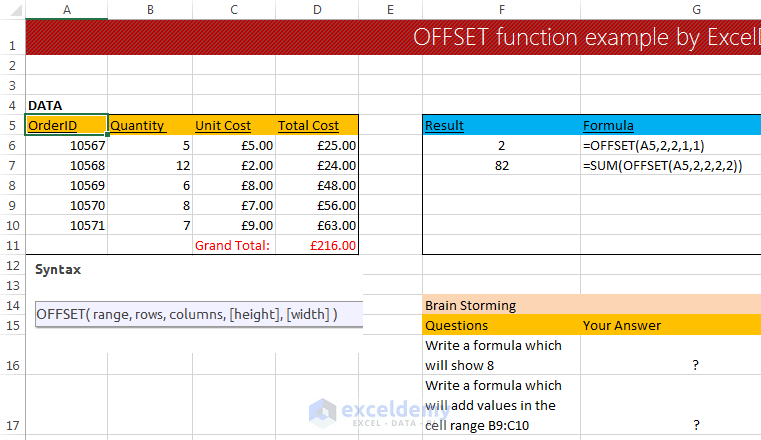
The OFFSET function in Excel is a powerful and versatile tool that allows you to return a range of cells that is a specified number of rows and columns from a starting reference. Think of it as a dynamic cell pointer that you can move around your spreadsheet. It’s especially useful for creating dynamic charts, formulas, and named ranges that automatically adjust to changing data. While seemingly simple, mastering the OFFSET function opens up a wide array of possibilities for advanced Excel usage.

Understanding the Syntax

The OFFSET function has the following syntax:

=OFFSET(reference, rows, cols, [height], [width])

Let’s break down each argument:

reference: This is the starting cell or range from which you want to offset. It’s the anchor point for the function. This must be a cell or a range of cells, and it’s crucial to choose the right reference to get the desired result.
rows: The number of rows to offset from the reference. A positive number moves down, a negative number moves up, and zero means no row offset.
cols: The number of columns to offset from the reference. A positive number moves right, a negative number moves left, and zero means no column offset.
[height]: (Optional) The height of the returned range, in number of rows. If omitted, it defaults to the height of the reference. If your reference is a single cell, the default height is 1.
[width]: (Optional) The width of the returned range, in number of columns. If omitted, it defaults to the width of the reference. If your reference is a single cell, the default width is 1.

It’s important to note that OFFSET *returns a reference*, not a value. This means you typically use it in conjunction with other functions like SUM, AVERAGE, COUNT, or even other OFFSET functions to extract and manipulate the data it points to.

Basic Examples

Let’s start with some basic examples to illustrate how OFFSET works:

Assume the following data in your Excel sheet:

        A     B     C     D 1   10    20    30    40 2   50    60    70    80 3   90   100   110   120 4  130   140   150   160

=OFFSET(A1, 1, 1) This starts at cell A1, moves down 1 row, and right 1 column. The result is cell B2, which contains the value 60.
=OFFSET(A1, 2, 0) This starts at cell A1, moves down 2 rows, and stays in the same column (0 columns offset). The result is cell A3, which contains the value 90.
=OFFSET(C2, -1, -2) This starts at cell C2, moves up 1 row, and left 2 columns. The result is cell A1, which contains the value 10.
=OFFSET(A1, 0, 0, 3, 2) This starts at cell A1, does not move (0 rows, 0 columns), and returns a range that is 3 rows high and 2 columns wide. The result is the range A1:B3, containing the values 10, 20, 50, 60, 90, and 100. Notice that `OFFSET` by itself doesn’t *display* these values. You’d typically use it within another function to work with this range.

Using OFFSET with Other Functions

The real power of OFFSET comes when you combine it with other Excel functions. Here are some common use cases:

1. Summing a Dynamic Range

Suppose you want to sum the values in the first three rows of column B. You could use the following formula:

=SUM(OFFSET(B1, 0, 0, 3, 1))

This starts at B1, offsets by 0 rows and 0 columns (so it stays at B1), and then creates a range that is 3 rows high and 1 column wide (B1:B3). The SUM function then adds up the values in this range.

Now, imagine you want to sum the values in the *last* three rows of column B, assuming you don’t know how many rows of data you have. You can use the COUNTA function to determine the number of filled rows and then use that in your OFFSET formula:

=SUM(OFFSET(B1, COUNTA(B:B)-3, 0, 3, 1))

Here’s how this works:

COUNTA(B:B) counts the number of non-empty cells in column B, including headers. Let’s say there are 5 rows of data.
COUNTA(B:B)-3 calculates 5 – 3 = 2. This is the number of rows to offset *down* from B1 to reach the beginning of the last three rows (B3 in this case).
OFFSET(B1, 2, 0, 3, 1) creates a range that starts at B3 and is 3 rows high and 1 column wide (B3:B5).
SUM then adds up the values in B3:B5.

2. Averaging a Moving Window

You can use OFFSET to calculate a moving average. For example, to calculate the average of the last 5 days of sales data, you could use a formula like this:

Assume sales data is in column C, starting from C2:

=AVERAGE(OFFSET(C2, COUNTA(C:C)-6, 0, 5, 1))

Similar to the previous example, COUNTA(C:C) counts the number of data entries in column C (including any header). We subtract 6 to move to the starting point for the average, use a height of 5 rows, and a width of 1 column. This effectively calculates the average of the previous 5 values.

3. Creating Dynamic Named Ranges

One of the most powerful uses of OFFSET is in creating dynamic named ranges. This allows you to define a name that refers to a range of cells that automatically adjusts as data is added or removed. Here’s how to do it:

Go to the “Formulas” tab in Excel.
Click on “Define Name”.
In the “New Name” dialog box:
- Enter a name for your range (e.g., “MyData”).
- In the “Refers to” field, enter an OFFSET formula.
Click “OK”.

For example, let’s say you have a list of products in column A and their corresponding prices in column B. You want to create a dynamic named range called “Prices” that always includes all the prices, regardless of how many products are added to the list.

In the “Refers to” field, you would enter the following formula (assuming the prices start in cell B2):

=OFFSET(Sheet1!B2,0,0,COUNTA(Sheet1!B:B)-1,1)

This formula does the following:

Sheet1!B2 is the starting reference point (the first price).
0,0 means no row or column offset.
COUNTA(Sheet1!B:B)-1 calculates the number of prices in column B (excluding the header). This becomes the height of the range. We subtract 1 because COUNTA counts the header in B1.
1 is the width of the range (1 column).

Now, you can use the named range “Prices” in other formulas. For example, to calculate the total value of all products, you could use:

=SUM(Prices)

The “Prices” range will automatically adjust as you add or remove products and their prices from columns A and B, respectively.

4. Extracting Data from a Table Dynamically

Imagine you have a table of sales data organized by month and product. You want to extract the sales figures for a specific product for the last six months. You can combine OFFSET with MATCH and INDEX to achieve this.

Let’s say the table looks like this:

        A         B        C        D        E        F        G 1  Month     Product1 Product2 Product3 Product4 Product5 Product6 2  Jan       100      150      200      250      300      350 3  Feb       110      160      210      260      310      360 4  Mar       120      170      220      270      320      370 5  Apr       130      180      230      280      330      380 6  May       140      190      240      290      340      390 7  Jun       150      200      250      300      350      400 8  Jul       160      210      260      310      360      410 9  Aug       170      220      270      320      370      420 10 Sep       180      230      280      330      380      430 11 Oct       190      240      290      340      390      440 12 Nov       200      250      300      350      400      450 13 Dec       210      260      310      360      410      460

Assume the product name you want to extract data for is in cell I1 (e.g., “Product3”). You want to get the last 6 months of sales data for that product. Here’s the formula:

=OFFSET(B1, COUNTA(A:A)-7, MATCH(I1,B1:G1,0)-1, 6, 1)

Let’s break it down:

B1 is the starting reference (the first data cell).
COUNTA(A:A)-7 calculates the number of rows to offset down. COUNTA(A:A) counts the number of months (including the header “Month”). Subtracting 7 gets you the starting row for the last 6 months (13 – 7 = 6, meaning start at row 6 relative to B1).
MATCH(I1,B1:G1,0)-1 finds the column corresponding to the product name in I1. MATCH returns the position of the product name within the range B1:G1. Subtracting 1 adjusts for the offset from column B. For example, if I1 contains “Product3”, MATCH returns 3, and subtracting 1 gives 2.
6, 1 defines the range to be 6 rows high (last 6 months) and 1 column wide.

This formula dynamically retrieves the sales figures for the specified product for the last six months, regardless of how many months of data are in the table.

Important Considerations and Potential Issues

Volatility: The OFFSET function is volatile. This means it recalculates whenever *any* cell in the worksheet changes, even if those changes are unrelated to the OFFSET formula. This can slow down your spreadsheet if you use many OFFSET formulas. Consider using INDEX and MATCH as alternatives when possible, as they are not volatile.
Error Handling: If your OFFSET formula results in a reference that is outside the boundaries of the worksheet, it will return a #REF! error. Pay close attention to the ‘rows’ and ‘cols’ arguments, especially when using negative offsets.
Clarity: Complex OFFSET formulas can be difficult to understand and debug. Use comments and descriptive cell names to make your formulas more readable and maintainable.
Alternatives: In many cases, the INDEX and MATCH functions provide a more efficient and less volatile alternative to OFFSET. Especially for looking up values in tables, INDEX and MATCH often offer better performance and readability.

In conclusion, the OFFSET function is a valuable tool for creating dynamic formulas and named ranges in Excel. By understanding its syntax and combining it with other functions, you can automate complex calculations and analyses. However, be mindful of its volatility and consider using alternative functions like INDEX and MATCH when appropriate.

761×440 offset function excel examples exceldemycom from www.exceldemy.com

752×546 excel offset function formula examples video from trumpexcel.com

1516×670 excel offset function excelfind from excelfind.com

321×205 excel offset function examples from www.listendata.com

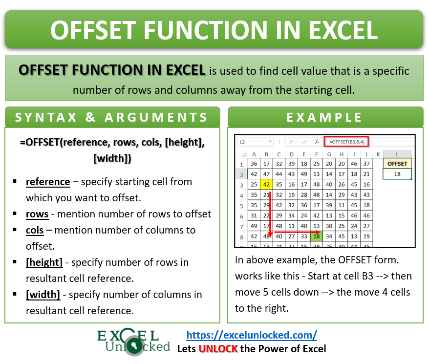876×745 offset function excel jump rows columns excel unlocked from excelunlocked.com

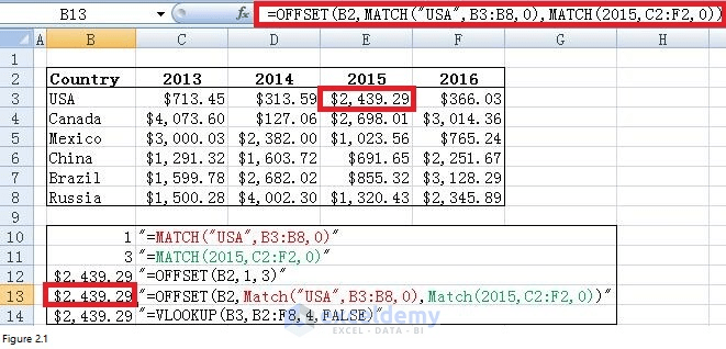661×318 offset function excel offset match combo dynamic range from www.exceldemy.com

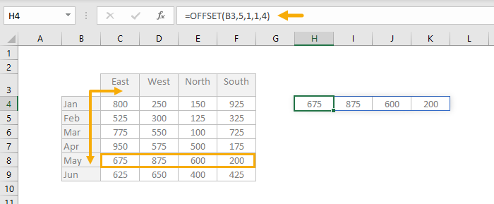700×289 excel offset function exceljet from exceljet.net

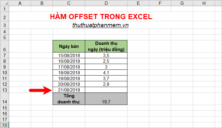730×422 offset function excel usage examples from tipsmake.com

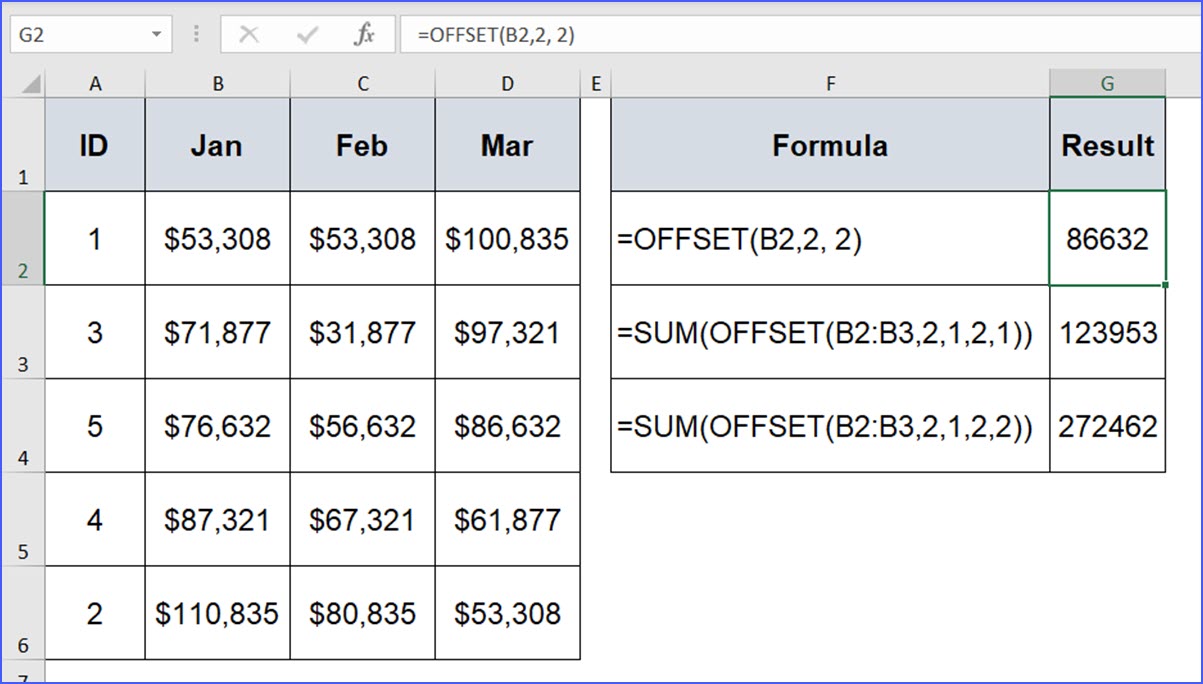1203×684 offset function excelnotes from excelnotes.com

604×367 offset function excel easy excel tutorial from www.excel-easy.com

700×332 offset function excel teachexcelcom from www.teachexcel.com

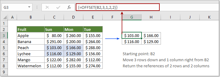726×254 offset function excel from www.extendoffice.com

1024×563 offset function excel solutions offset functions from yodalearning.com

How To Use The Offset Function In Excel With Examples was posted in January 26, 2026 at 4:33 am. If you wanna have it as yours, please click the Pictures and you will go to click right mouse then Save Image As and Click Save and download the How To Use The Offset Function In Excel With Examples Picture.. Don’t forget to share this picture with others via Facebook, Twitter, Pinterest or other social medias! we do hope you'll get inspired by ExcelKayra... Thanks again! If you have any DMCA issues on this post, please contact us!