How To Calculate Loan Amortization In Excel With Formulas
How To Calculate Loan Amortization In Excel With Formulas - There are a lot of affordable templates out there, but it can be easy to feel like a lot of the best cost a amount of money, require best special design template. Making the best template format choice is way to your template success. And if at this time you are looking for information and ideas regarding the How To Calculate Loan Amortization In Excel With Formulas then, you are in the perfect place. Get this How To Calculate Loan Amortization In Excel With Formulas for free here. We hope this post How To Calculate Loan Amortization In Excel With Formulas inspired you and help you what you are looking for.
“`html
Calculating Loan Amortization in Excel: A Step-by-Step Guide
Understanding loan amortization is crucial for anyone taking out a loan, whether it’s a mortgage, auto loan, or personal loan. Amortization refers to the process of gradually paying off a loan over time through regular payments, each containing a portion allocated to principal and a portion allocated to interest. Excel is a powerful tool for creating loan amortization schedules, allowing you to visualize how your loan balance decreases over the repayment period. This guide provides a detailed, step-by-step explanation of how to calculate loan amortization in Excel using formulas.
Key Loan Parameters
Before diving into the formulas, let’s define the key parameters needed to create an amortization schedule:
- Loan Amount (Principal): The total amount borrowed.
- Interest Rate: The annual interest rate charged on the loan.
- Loan Term (in Years): The duration of the loan in years.
- Payments per Year: The number of payments made each year (e.g., 12 for monthly payments).
- Payment Amount: The fixed payment amount for each period.
Setting Up Your Excel Worksheet
First, organize your Excel worksheet to clearly display these parameters. Here’s a suggested layout:
| Label | Cell | Example Value |
|---|---|---|
| Loan Amount | B1 | $100,000 |
| Interest Rate (Annual) | B2 | 5% |
| Loan Term (Years) | B3 | 30 |
| Payments per Year | B4 | 12 |
| Payment Amount | B5 | (Calculated Below) |
Now, let’s calculate the payment amount using the PMT function. In cell B5, enter the following formula:
=PMT(B2/B4, B3*B4, B1)
Explanation:
B2/B4: Divides the annual interest rate (B2) by the number of payments per year (B4) to get the periodic interest rate.B3*B4: Multiplies the loan term in years (B3) by the number of payments per year (B4) to get the total number of payments.B1: The loan amount (present value).
The PMT function returns the payment amount, which will be a negative value since it represents an outflow of cash. You can wrap the formula in a - (minus sign) to display it as a positive value: =-PMT(B2/B4, B3*B4, B1)
Creating the Amortization Schedule
Now, create the amortization schedule table. Start by setting up the following column headers:
| Period | Beginning Balance | Payment | Interest Paid | Principal Paid | Ending Balance |
|---|---|---|---|---|---|
| Column A | Column B | Column C | Column D | Column E | Column F |
Let’s populate the rows with the necessary formulas. Assume the schedule starts in row 7.
Row 7 (First Period)
- Period (A7): Enter
1. - Beginning Balance (B7): Enter
=B1(the loan amount). - Payment (C7): Enter
=B$5. Note the use of the$signs. This creates an absolute reference, ensuring that this cell always refers to the payment amount calculated in cell B5. - Interest Paid (D7): Enter
=B7*(B$2/B$4). This calculates the interest paid for the first period by multiplying the beginning balance by the periodic interest rate. Again, use absolute references for the interest rate and payments per year. - Principal Paid (E7): Enter
=C7-D7. This calculates the principal paid by subtracting the interest paid from the total payment. - Ending Balance (F7): Enter
=B7-E7. This calculates the ending balance by subtracting the principal paid from the beginning balance.
Row 8 and Beyond
Now, let’s populate the remaining rows by copying the formulas from row 7. However, the “Period” and “Beginning Balance” formulas require slight adjustments.
- Period (A8): Enter
=A7+1. This increments the period number. - Beginning Balance (B8): Enter
=F7. The beginning balance for the current period is the ending balance from the previous period.
Now, select cells C7 through F7 and drag the fill handle (the small square at the bottom right of the selection) down to the desired number of periods. For a 30-year loan with monthly payments, you’ll drag it down 360 rows (30 years * 12 months/year).
You can then copy the formula from A8 (=A7+1) and paste it down to the same number of rows, completing the “Period” column.
Handling the Final Payment
It’s highly likely that the ending balance in the final period won’t be exactly zero due to rounding errors. To correct this, we can adjust the formula for the principal paid in the final period.
First, identify the row containing the last period (e.g., row 366 if you have 360 payments plus the header row and the initial data row). In the “Ending Balance” column (Column F) of this row, enter 0.
Then, in the “Principal Paid” column (Column E) of the last period’s row, enter =B366 (referencing the beginning balance of that period). This ensures that the principal paid is exactly equal to the remaining balance, resulting in a zero ending balance.
Finally, adjust the “Payment” amount in the final period. In cell C366, enter =D366+E366. This recalculates the final payment to be the sum of the interest paid and the principal paid in that period.
Conditional Formatting (Optional)
To visually highlight the amortization schedule, you can use conditional formatting. For example, you can apply data bars to the “Interest Paid” and “Principal Paid” columns to visualize the proportion of each payment allocated to each component. Select the data in the “Interest Paid” column (excluding the header), go to “Conditional Formatting” -> “Data Bars”, and choose a style. Repeat for the “Principal Paid” column.
Summary
By following these steps, you can create a comprehensive loan amortization schedule in Excel. This schedule will provide valuable insights into how your loan is paid off over time, helping you understand the breakdown of each payment and the remaining loan balance. Remember to double-check your formulas and adjust them as needed based on your specific loan terms.
Important Considerations
- Rounding: Excel’s rounding can sometimes lead to slight discrepancies. Adjusting the final payment is usually sufficient to correct this.
- Extra Payments: This schedule assumes regular, consistent payments. If you make extra payments, you’ll need to modify the schedule accordingly, which can involve more complex formulas or VBA scripting.
- Variable Interest Rates: This schedule is designed for fixed-rate loans. For variable-rate loans, you’ll need to update the interest rate periodically and recalculate the amortization schedule.
“`
 1274×785 loan amortization loan amortization templates from myexceltemplates.com
  707×461 loan amortization excel template exceldatapro from exceldatapro.com
 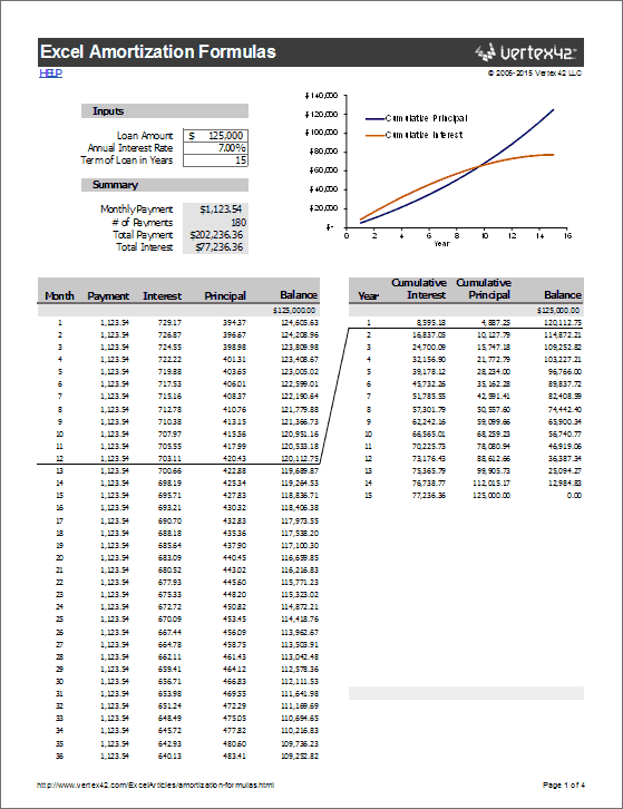 559×726 amortization formulas excel from www.vertex42.com
  604×707 loan amortization schedule excel step step tutorial from www.excel-easy.com
  1024×526 loan amortization equation tessshebaylo from www.tessshebaylo.com
  626×731 loan amortization schedule calculator from www.vertex42.com
  1368×974 loan amortizationxls from www.excelcalcs.com
  1024×865 loan amortization schedule excel ordnur from ordnur.com
  728×546 prepare amortization schedule excel steps from www.wikihow.com
 How To Calculate Loan Amortization In Excel With Formulas was posted in September 17, 2025 at 1:26 am. If you wanna have it as yours, please click the Pictures and you will go to click right mouse then Save Image As and Click Save and download the How To Calculate Loan Amortization In Excel With Formulas Picture.. Don’t forget to share this picture with others via Facebook, Twitter, Pinterest or other social medias! we do hope you'll get inspired by ExcelKayra... Thanks again! If you have any DMCA issues on this post, please contact us!