How To Make A Gantt Chart In Excel For Project Timelines
How To Make A Gantt Chart In Excel For Project Timelines - There are a lot of affordable templates out there, but it can be easy to feel like a lot of the best cost a amount of money, require best special design template. Making the best template format choice is way to your template success. And if at this time you are looking for information and ideas regarding the How To Make A Gantt Chart In Excel For Project Timelines then, you are in the perfect place. Get this How To Make A Gantt Chart In Excel For Project Timelines for free here. We hope this post How To Make A Gantt Chart In Excel For Project Timelines inspired you and help you what you are looking for.
“`html
Creating Gantt Charts in Excel for Project Timelines
Gantt charts are powerful visual tools for project management, providing a clear overview of tasks, their durations, and dependencies. While dedicated project management software offers advanced Gantt chart features, Excel provides a simple and accessible way to create basic Gantt charts for smaller projects or quick visualizations. This guide walks you through several methods for creating Gantt charts in Excel, catering to different levels of complexity and desired visual customization.
Method 1: Basic Bar Chart Gantt Chart (Using Stacked Bar Chart)
This method is the most common and straightforward way to create a Gantt chart in Excel. It leverages the stacked bar chart feature to represent tasks and their durations.
Steps:
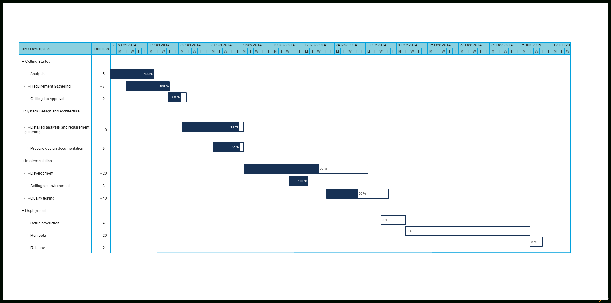
- Prepare Your Data: Organize your project data in a clear table format. You’ll need at least three columns:
- Task Name: The name or description of each task.
- Start Date: The date on which the task is scheduled to begin.
- Duration (Days): The number of days the task is expected to take. Alternatively, you could use ‘End Date’ instead of ‘Duration’ and calculate the duration using a formula.
Example:
Task Name Start Date Duration (Days) Project Planning 1/1/2024 5 Requirements Gathering 1/8/2024 7 Design Phase 1/17/2024 10 Development 1/31/2024 15 Testing 2/21/2024 7 - Add a ‘Start Day’ Column: This column will calculate the number of days between your project’s start date and each task’s start date. This is crucial for positioning the bars correctly on the chart.
- In a new column (e.g., “Start Day”), enter the following formula in the first row (assuming your first task’s start date is in cell B2, and you designate cell B2 as your project’s start date). The formula locks the project start date cell so that when you drag, all calculations refer to it.
=B2-$B$2 - Format the ‘Start Day’ column as a number (General or Number format).
- Drag the formula down to apply it to all tasks.
- In a new column (e.g., “Start Day”), enter the following formula in the first row (assuming your first task’s start date is in cell B2, and you designate cell B2 as your project’s start date). The formula locks the project start date cell so that when you drag, all calculations refer to it.
- Insert a Stacked Bar Chart:
- Select the ‘Task Name’ column and the ‘Start Day’ column. Hold down the Ctrl key (or Cmd key on Mac) while selecting to select non-adjacent columns.
- Go to the “Insert” tab on the Excel ribbon.
- In the “Charts” group, click the “Insert Bar or Column Chart” dropdown.
- Choose “Stacked Bar.”
- Add the ‘Duration’ Data Series:
- Right-click on the chart and select “Select Data.”
- In the “Select Data Source” dialog box, click “Add.”
- In the “Edit Series” dialog box:
- In the “Series name” field, you can type “Duration” (optional).
- In the “Series values” field, select the range of cells containing the ‘Duration’ values (excluding the column header).
- Click “OK” twice to close the dialog boxes.
- Format the Chart:
- Invert Task Order: The task names will likely appear in reverse order on the vertical axis. To correct this:
- Click on the vertical axis (Task Names).
- Right-click and select “Format Axis.”
- In the “Format Axis” pane, under “Axis Options,” check the “Categories in reverse order” box.
- Remove the ‘Start Day’ Bars: The ‘Start Day’ bars represent the delay before a task begins. To make them invisible:
- Click on one of the blue bars (the ‘Start Day’ series). This should select all bars in that series.
- Right-click and select “Format Data Series.”
- In the “Format Data Series” pane, go to the “Fill & Line” tab.
- Under “Fill,” select “No fill.”
- Under “Border,” select “No line.”
- Format the Duration Bars: Customize the color and appearance of the duration bars to improve readability.
- Click on one of the orange bars (the ‘Duration’ series). This should select all bars in that series.
- Right-click and select “Format Data Series.”
- In the “Format Data Series” pane, go to the “Fill & Line” tab.
- Adjust the “Fill” color, “Border” color, and “Border” width as desired.
- Adjust the Horizontal Axis: The horizontal axis might not start at the project start date. Adjust it as follows:
- Click on the horizontal axis (dates).
- Right-click and select “Format Axis.”
- In the “Format Axis” pane, under “Axis Options”:
- Set the “Minimum” value to the numerical value corresponding to the project’s start date. You can find this value by formatting the Start Date cell as “Number” and noting the resulting number. Alternatively, use the `DATE` function. The minimum value would be the number value of `DATE(2024,1,1)` if your project started 1/1/2024.
- Set the “Maximum” value similarly based on the project’s end date or a desired end date range for the chart.
- Adjust the “Units” for the axis. Major units control the spacing between the larger gridlines. Minor units control the spacing between smaller gridlines. Try “Days” or “Weeks” for major units.
- Add Gridlines and Labels (Optional): Add horizontal gridlines for easier reading. Add labels for milestones or important deadlines.
- Chart Title and Axis Titles: Add a descriptive chart title and labels for the horizontal and vertical axes.
- Invert Task Order: The task names will likely appear in reverse order on the vertical axis. To correct this:
Method 2: Using Conditional Formatting
This method offers more visual control and allows you to highlight specific periods or milestones directly on the worksheet. However, it’s less interactive than a chart-based Gantt chart.
Steps:
- Prepare Your Data: Similar to the previous method, organize your data with columns for ‘Task Name’, ‘Start Date’, and ‘Duration (Days)’. Optionally include an ‘End Date’ column, calculated as `=Start Date + Duration – 1`.
- Create a Date Range Header Row: In a row above your task data (e.g., row 1), enter the project start date in the first cell (e.g., B1). Then, in the next cell (C1), enter the formula `=B1+1`. Drag this formula across the row to create a series of consecutive dates that cover the entire project timeline. Format the date range row to display only the day number or month, making it more compact. Adjust column widths to fit the day or month display.
- Apply Conditional Formatting:
- Select the range of cells where you want the Gantt chart to appear (excluding the header row with dates). For example, if your task names are in column A starting at A2, and your date range starts at B1 and extends to, say, AA1, then select the range B2:AA[last task row number].
- Go to the “Home” tab on the Excel ribbon.
- In the “Styles” group, click “Conditional Formatting” and then “New Rule.”
- In the “New Formatting Rule” dialog box, select “Use a formula to determine which cells to format.”
- Enter the following formula (adjust cell references to match your actual data):
=AND(B$1>=$C2,B$1<=$D2)- `B$1`: Refers to the date in the header row. The `$` before `1` ensures that the row remains fixed when the rule is applied to other rows.
- `$C2`: Refers to the start date for the task. The `$` before `C` ensures that the column remains fixed when the rule is applied to other columns.
- `$D2`: Refers to the end date for the task. If you use 'Duration', calculate 'End Date' and use that column. The `$` before `D` ensures that the column remains fixed when the rule is applied to other columns.
- Click the "Format" button and choose the desired fill color for the Gantt chart bars.
- Click "OK" twice to close the dialog boxes.
- Customize Appearance (Optional): Adjust column widths, add borders, or use different colors to enhance the visual clarity.
Method 3: Using a Scatter Plot and Error Bars
This method, while more complex to set up, provides greater flexibility in customizing the appearance and adding advanced features like task dependencies (with some manual adjustments).
Steps:
- Prepare Your Data: You'll need 'Task Name', 'Start Date', 'Duration (Days)', and 'End Date' (calculated from 'Start Date' and 'Duration'). You'll also need to convert the dates to numerical values for the scatter plot to work. You can add a column called "Start Value" and calculate it as the numerical representation of the Start Date using `=Start Date`. Do the same for "End Value."
- Insert a Scatter Plot:
- Select the 'Task Name' column and the 'Start Value' column (or 'End Value', depending on how you want to plot it initially).
- Go to the "Insert" tab and choose a Scatter plot without lines (a simple scatter plot with markers).
- Add Error Bars:
- Click on the scatter plot.
- Go to the "Chart Design" tab (or "Chart Tools > Design").
- Click "Add Chart Element," then "Error Bars," then "More Error Bar Options."
- In the "Format Error Bars" pane:
- Select "Minus" direction.
- Choose "Percentage" and set the percentage to 100% (to extend the error bars fully to the left from the data point). If using 'End Value' for initial plot, choose "Plus" direction.
- Click the Error Bars icon again and go back to "More Error Bar Options." Under the "Error Amount" Section, choose Custom and Specify a value: for Negative Error value choose `='Sheet1'!$D2:$D6` where your durations are stored. Make sure to change the range according to your data range. For positive, leave it to 0.
- In the "Format Error Bars" pane, go to the "Fill & Line" tab and customize the color, width, and cap type of the error bars to resemble Gantt chart bars.
- Format the Chart: Adjust the axis scales, remove markers, invert the task order, and add labels, similar to Method 1. The primary difference is you're working with a scatter plot and error bars instead of stacked bars. The X-axis will be based on the numerical date values.
- Customize Further (Optional): Add connecting lines to show dependencies (manually drawn), adjust the marker size, and use data labels to display additional information.
Tips and Considerations:
* **Date Formatting:** Ensure your date columns are properly formatted as dates in Excel. * **Customization:** Experiment with different colors, fills, and borders to create a visually appealing and informative Gantt chart. * **Dynamic Updates:** To make your Gantt chart more dynamic, use formulas and named ranges to automatically update the chart when the underlying data changes. * **Complexity:** For complex projects with numerous tasks and dependencies, consider using dedicated project management software for more robust Gantt chart features. * **Milestones:** Represent milestones as diamond shapes or distinct markers on the chart for easy identification. * **Critical Path:** Visually highlight the critical path (the sequence of tasks that directly affects the project's completion date) for better project focus. * **Zooming:** Adjust the horizontal axis scale to zoom in or out on specific periods of the project timeline.
By mastering these methods, you can effectively create Gantt charts in Excel to visualize project timelines, track progress, and improve project management efficiency.
```
 1965×975 gantt chart templates instantly create project timelines high from db-excel.com
  1280×720 gantt chart project timeline template excel infoupdateorg from infoupdate.org
  1485×584 project timeline template gantt chart project excel dbbool from dbbool.weebly.com
  1024×1024 excel gantt chart flexible project spreadsheet luxtemplates from luxtemplates.com
  790×711 visualizing project timelines gantt chart excel template from slidesdocs.com
  1299×444 creating project timeline gantt chart ms excel excel zoom from excelzoom.com
  1164×668 project timeline excel template gantt chart from mungfali.com
  1273×758 project timeline gantt chart excel template template resume from www.contrapositionmagazine.com
  1024×462 gantt excel timeline gantt excel from ganttxl.com
  1280×720 excel template gantt chart project time chart from smartofficetemplates.myinstamojo.com
  2550×2188 project timeline gantt chart excel doctemplates from doctemplates.us
  1248×680 excel timeline gantt chart excel timeline template from ganttchartsexcel.z21.web.core.windows.net
  1200×741 gantt chart visualizing project timelines progress excel template from slidesdocs.com
  1760×1140 project timeline gantt chart template excel google sheets from www.template.net
  1915×705 project timeline template list template gantt chart templates from www.pinterest.de
  1920×1040 gantt chart project plan excel from uniformsoftware.com
  700×472 visualizing project timeline formula gantt chart excel template from pikbest.com
  1266×593 project timeline gantt chart excel model eloquens from www.eloquens.com
  1506×944 timeline gantt chart excel template hot sex picture from www.hotzxgirl.com
  2048×1142 gantt chart excel save time spreadsheet gantt from business-docs.co.uk
  1711×1059 project plan gantt chart excel template excel templates from www.exceltemplate123.us
  4640×2612 drawing gantt chart excel gantt chart template word from ganttchartsexcel.z21.web.core.windows.net
  1500×1125 create project timeline gantt chart excel printable from tupuy.com
  800×600 beautiful work gantt chart timeline template excel project plan from nobodyjoint15.pythonanywhere.com
  1920×1080 simple excel gantt chart automated project timeline microsoft excel from www.etsy.com
  700×442 creating gantt chart illustrate annual project timeline excel from pikbest.com
  700×558 creating effective project timeline gantt chart excel from pikbest.com
  700×426 creating project timeline gantt chart ultimate guide excel from pikbest.com
  1430×1073 timeline gantt chart excel printable from tupuy.com
 How To Make A Gantt Chart In Excel For Project Timelines was posted in September 26, 2025 at 7:12 am. If you wanna have it as yours, please click the Pictures and you will go to click right mouse then Save Image As and Click Save and download the How To Make A Gantt Chart In Excel For Project Timelines Picture.. Don’t forget to share this picture with others via Facebook, Twitter, Pinterest or other social medias! we do hope you'll get inspired by ExcelKayra... Thanks again! If you have any DMCA issues on this post, please contact us!