How To Use Iferror Function To Clean Data In Excel
How To Use Iferror Function To Clean Data In Excel - There are a lot of affordable templates out there, but it can be easy to feel like a lot of the best cost a amount of money, require best special design template. Making the best template format choice is way to your template success. And if at this time you are looking for information and ideas regarding the How To Use Iferror Function To Clean Data In Excel then, you are in the perfect place. Get this How To Use Iferror Function To Clean Data In Excel for free here. We hope this post How To Use Iferror Function To Clean Data In Excel inspired you and help you what you are looking for.
“`html
Cleaning Data in Excel with the IFERROR Function
Excel is a powerful tool for data analysis, but raw data is rarely perfect. Cleaning and transforming data is a crucial step before any meaningful analysis can be performed. The `IFERROR` function in Excel is a versatile tool that can significantly aid in this process by gracefully handling errors and allowing you to replace them with more desirable values. This guide will delve into the practical applications of `IFERROR` for data cleaning, covering various scenarios and providing clear examples.
Understanding the IFERROR Function
The `IFERROR` function has a simple syntax:
=IFERROR(value, value_if_error)- value: The expression or formula you want to evaluate.
- value_if_error: The value you want to return if the `value` argument results in an error.
The function works by first evaluating the `value` argument. If the evaluation is successful and doesn’t produce an error, `IFERROR` returns the result of the `value` argument. However, if the evaluation results in an error of any kind (e.g., `#DIV/0!`, `#VALUE!`, `#REF!`, `#NAME?`, `#NUM!`, `#N/A`, or `#NULL!`), then `IFERROR` returns the `value_if_error` argument. This allows you to catch and handle potential errors proactively.
Common Data Cleaning Scenarios and IFERROR Applications
-
Handling Division by Zero Errors (#DIV/0!)
Division by zero is a common error in spreadsheets, especially when dealing with ratios or calculations involving potentially zero denominators. `IFERROR` provides a clean way to prevent these errors from propagating through your calculations and displaying unsightly `#DIV/0!` errors. For instance, imagine you have sales data and units sold, and you want to calculate the price per unit. Some units might have no sales (units sold = 0).
Example: Column A contains ‘Sales’ and Column B contains ‘Units Sold’. You want to calculate ‘Price per Unit’ in Column C.
Without `IFERROR`, you might use the formula `=A2/B2` in cell C2. This would result in a `#DIV/0!` error whenever B2 is zero.
Using `IFERROR`, you can replace this with the formula `=IFERROR(A2/B2, 0)`. This formula does the following:
- If `A2/B2` results in a valid number, the result is shown.
- If `A2/B2` results in a `#DIV/0!` error (because B2 is zero), the formula returns 0.
You can replace the zero with other values or even text. For example, `=IFERROR(A2/B2, “N/A”)` will display “N/A” in cells where division by zero occurs.
-
Dealing with #N/A Errors (Missing Data)
The `#N/A` error typically arises when a function, such as `VLOOKUP` or `MATCH`, cannot find a matching value. This often indicates missing data or inconsistencies in your data sets. Using `IFERROR` allows you to replace these missing values with more manageable substitutes.
Example: You have a list of customer IDs in Column A and their corresponding names in a separate table. You use `VLOOKUP` to retrieve the customer names into Column B.
Without `IFERROR`, the formula in B2 might be `=VLOOKUP(A2,Sheet2!$A$1:$B$100,2,FALSE)`. If the `VLOOKUP` function doesn’t find the `A2` customer ID in `Sheet2!$A$1:$A$100`, it returns `#N/A`.
Using `IFERROR`, you can use the formula `=IFERROR(VLOOKUP(A2,Sheet2!$A$1:$B$100,2,FALSE), “Customer Not Found”)`. This:
- Retrieves the customer name if the ID is found.
- Displays “Customer Not Found” if the ID isn’t in the lookup table, replacing the `#N/A` error.
Instead of displaying text, you could also replace the `#N/A` with a numerical value, such as 0, or leave it blank (`””`). The choice depends on how you intend to use the data.
-
Handling Errors in Complex Formulas
When you create complex formulas that combine multiple functions, the chance of encountering an error increases. `IFERROR` can be used to wrap these complex formulas and handle any potential errors that may arise.
Example: You have a formula that calculates a discount based on multiple conditions. This formula might involve nested `IF` statements and other calculations.
Let’s say your complex discount calculation formula is in cell D2 and might produce errors due to data inconsistencies or calculation problems.
You can use `IFERROR(D2, 0)` to replace any error in D2 with a zero discount. This prevents the error from affecting subsequent calculations and provides a default value.
You can also use `IFERROR` to provide more informative error messages. For example, `=IFERROR(D2, “Error in Discount Calculation”)` will display this text if an error occurs in the discount calculation formula. This can help you quickly identify and troubleshoot the problem.
-
Cleaning Data Imported from External Sources
Data imported from external sources (e.g., databases, CSV files) often contains inconsistencies or errors. Using `IFERROR` during the import or immediately after can help clean up this data.
Example: You import a CSV file containing customer information. Some fields might contain invalid characters or be in the wrong format, leading to errors during data conversion.
Suppose Column A contains customer ages, but some entries are text instead of numbers. You can use the formula `=IFERROR(VALUE(A2),0)` in column B to convert the text values to zero and valid numeric ages to their correct values. The `VALUE` function attempts to convert text to a number, and `IFERROR` catches the resulting `#VALUE!` error if the conversion fails.
By using `IFERROR` during data import, you can ensure that your data is consistent and ready for analysis.
-
Validating Data Entry
While `IFERROR` is primarily used for handling existing errors, it can also be incorporated into data validation rules to proactively prevent errors from being entered in the first place.
Example: You have a cell where users are supposed to enter a percentage value between 0 and 1. You can use data validation to ensure that only valid percentages are entered.
- Select the cell or range of cells where you want to apply the validation.
- Go to the “Data” tab on the Excel ribbon and click “Data Validation.”
- In the “Settings” tab, choose “Custom” from the “Allow” dropdown.
- Enter a formula in the “Formula” box that uses IFERROR and a logical test. For example, to ensure that the entered value is a number between 0 and 1, you could use:
=IFERROR(AND(A1>=0, A1<=1, ISNUMBER(A1)), FALSE) - In the "Error Alert" tab, customize the error message that will be displayed if the validation fails.
This formula works by first checking if the value is a number (`ISNUMBER(A1)`). Then, it checks if the number is between 0 and 1 (`AND(A1>=0, A1<=1)`). If either of these conditions is false, the `AND` function returns `FALSE`. The `IFERROR` function catches any errors that might occur (e.g., if the cell contains text) and also returns `FALSE`. Thus, only valid percentages will be allowed.
Best Practices When Using IFERROR
- Be Specific: Avoid using `IFERROR` as a blanket solution for all errors. Try to understand the potential sources of errors and target your `IFERROR` formulas accordingly. Overuse of `IFERROR` can mask underlying problems with your data or formulas.
- Choose Meaningful Replacement Values: Select a `value_if_error` that makes sense in the context of your data. Sometimes 0 is appropriate, while other times "N/A" or a blank cell (`""`) is more suitable.
- Document Your Use: Add comments to your formulas to explain why you are using `IFERROR` and what the `value_if_error` represents. This will make your spreadsheet easier to understand and maintain.
- Test Thoroughly: After implementing `IFERROR` formulas, test them with various data inputs to ensure they are working as expected. Pay particular attention to edge cases and scenarios that might trigger errors.
- Consider Alternatives: While `IFERROR` is convenient, consider alternative approaches like using conditional statements (`IF`, `IFS`) or dedicated error-handling functions (like `ISERROR`, `ISNA`, `ISBLANK`) for more granular control and error analysis.
Conclusion
The `IFERROR` function is an indispensable tool for cleaning data in Excel. By gracefully handling errors and replacing them with appropriate values, you can improve the accuracy, readability, and usability of your spreadsheets. By understanding the different scenarios in which `IFERROR` can be applied and following best practices, you can effectively clean your data and unlock its full potential for analysis and decision-making.
```
 1281×662 excel iferror function excelfind from excelfind.com
 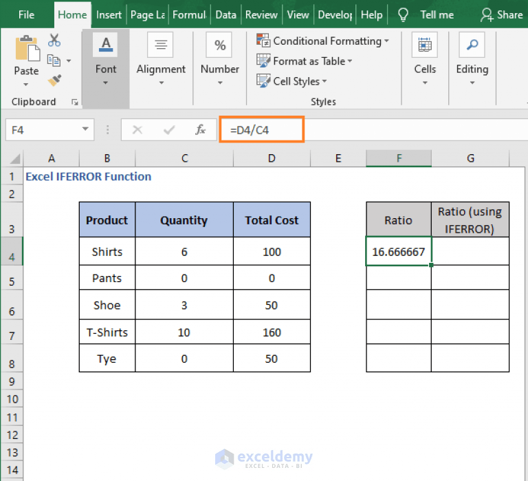 768×699 iferror function excel examples exceldemy from www.exceldemy.com
  876×717 iferror function excel remove excel error excel unlocked from excelunlocked.com
 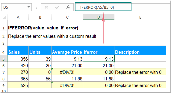 571×310 excel iferror function from www.extendoffice.com
 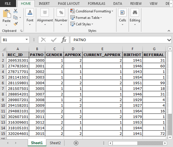 562×479 iferror function excel from www.exceltip.com
 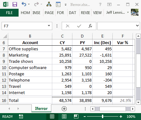 448×384 clean reports iferror excel university from www.excel-university.com
  735×499 handle errors excel iferror function examples from www.wallstreetmojo.com
  1100×514 iferror function excel examples geeksforgeeks from www.geeksforgeeks.org
 How To Use Iferror Function To Clean Data In Excel was posted in September 9, 2025 at 1:09 am. If you wanna have it as yours, please click the Pictures and you will go to click right mouse then Save Image As and Click Save and download the How To Use Iferror Function To Clean Data In Excel Picture.. Don’t forget to share this picture with others via Facebook, Twitter, Pinterest or other social medias! we do hope you'll get inspired by ExcelKayra... Thanks again! If you have any DMCA issues on this post, please contact us!