How To Use Iferror Function To Handle Errors In Excel Formulas
How To Use Iferror Function To Handle Errors In Excel Formulas - There are a lot of affordable templates out there, but it can be easy to feel like a lot of the best cost a amount of money, require best special design template. Making the best template format choice is way to your template success. And if at this time you are looking for information and ideas regarding the How To Use Iferror Function To Handle Errors In Excel Formulas then, you are in the perfect place. Get this How To Use Iferror Function To Handle Errors In Excel Formulas for free here. We hope this post How To Use Iferror Function To Handle Errors In Excel Formulas inspired you and help you what you are looking for.
Using IFERROR in Excel: A Comprehensive Guide to Error Handling
Excel is a powerful tool for data analysis and manipulation, but sometimes formulas can return errors. These errors can disrupt your workflow and make your spreadsheets look unprofessional. Fortunately, Excel provides the `IFERROR` function to gracefully handle these errors, replacing them with a value you specify.
What is the IFERROR Function?
The `IFERROR` function is a logical function that checks if a formula evaluates to an error and, if so, returns a specified value. The syntax is straightforward:
=IFERROR(value, value_if_error)- value: The expression or formula you want to evaluate.
- value_if_error: The value you want to return if the `value` argument results in an error.
The `IFERROR` function can handle various error types, including:
- `#DIV/0!` (Division by zero)
- `#N/A` (Value not available)
- `#NAME?` (Unrecognized name in formula)
- `#NULL!` (Intersection of two ranges does not intersect)
- `#NUM!` (Problem with a number in a formula)
- `#REF!` (Invalid cell reference)
- `#VALUE!` (Wrong type of argument or operand)
Basic Usage Examples
Example 1: Handling Division by Zero
Suppose you have a formula that divides one cell by another (e.g., `A2/B2`). If `B2` is zero, the formula will return `#DIV/0!`. To prevent this, use `IFERROR`:
=IFERROR(A2/B2, 0)This formula will return the result of `A2/B2` if it’s valid. If `B2` is zero, it will return `0` instead of the error.
Example 2: Handling #N/A Errors with VLOOKUP
`VLOOKUP` is a common function for finding data in a table. If `VLOOKUP` can’t find the lookup value, it returns `#N/A`. Use `IFERROR` to return a more user-friendly message or a default value:
=IFERROR(VLOOKUP(D2, A:B, 2, FALSE), "Not Found")Here, `VLOOKUP` searches for the value in `D2` within the range `A:B`. If the value isn’t found, `IFERROR` will return “Not Found” instead of `#N/A`.
Example 3: Returning an Empty String
Sometimes, you might want to leave a cell blank if an error occurs. You can achieve this by using an empty string (“”) as the `value_if_error`:
=IFERROR(C2*D2, "")This formula calculates the product of `C2` and `D2`. If either cell contains text or results in an error during multiplication, the cell will display an empty string, effectively appearing blank.
Advanced Usage and Considerations
Nesting IFERROR Functions
You can nest `IFERROR` functions to handle multiple potential error scenarios. This is useful when a formula relies on other formulas that might also generate errors.
=IFERROR(VLOOKUP(E2, A:B, 2, FALSE), IFERROR(HLOOKUP(E2, C:D, 2, FALSE), "Value Not Available"))This formula first tries `VLOOKUP`. If `VLOOKUP` returns an error, it then tries `HLOOKUP`. If `HLOOKUP` also returns an error, it finally returns “Value Not Available”.
Using IFERROR with INDEX and MATCH
`INDEX` and `MATCH` are powerful functions used together for dynamic lookups. `IFERROR` can be used to handle scenarios where the `MATCH` function doesn’t find a match.
=IFERROR(INDEX(B1:B10, MATCH(F2, A1:A10, 0)), "Item Not Found")This formula uses `MATCH` to find the row number where the value in `F2` is found within the range `A1:A10`. Then, `INDEX` retrieves the corresponding value from the range `B1:B10`. If `MATCH` doesn’t find a match, `IFERROR` returns “Item Not Found”.
Improving Performance with Caution
While `IFERROR` is convenient, it can potentially hide issues in your formulas. It’s crucial to understand why an error is occurring and address the underlying problem whenever possible. Overuse of `IFERROR` can also mask calculation errors and make debugging more difficult.
Furthermore, using `IFERROR` repeatedly within a large spreadsheet can impact performance, as it requires Excel to evaluate the first argument even when no error is present. Consider alternative approaches, like conditional formatting or data validation, if performance becomes an issue.
Handling Specific Error Types
Sometimes, you might want to handle specific error types differently. While `IFERROR` handles all errors, you can use a combination of `ISERROR`, `ISNA`, `ISNUMBER`, `ISTEXT` and other `IS` functions with the `IF` function to create more nuanced error handling.
=IF(ISNA(VLOOKUP(G2, A:B, 2, FALSE)), "Data Unavailable", VLOOKUP(G2, A:B, 2, FALSE))This formula specifically checks for `#N/A` errors returned by `VLOOKUP`. If an `#N/A` error is found, it returns “Data Unavailable”. Otherwise, it returns the result of the `VLOOKUP` formula.
Alternatives to IFERROR
While `IFERROR` is the most direct approach for handling errors, other options might be more appropriate in certain situations:
- Data Validation: Prevent users from entering invalid data that could cause errors in the first place. For example, you could restrict data entry in a cell to only numbers or specific values.
- Conditional Formatting: Highlight cells containing errors to easily identify and correct them.
- Array Formulas: In some cases, using array formulas can avoid errors that might occur when dealing with individual cells.
- Error Checking Options: Excel has built-in error checking options that can help you identify and resolve errors. Go to `File > Options > Formulas > Error Checking` to configure these options.
Best Practices
- Use `IFERROR` judiciously: Don’t use it as a “catch-all” for poorly designed formulas. Try to understand and fix the underlying causes of errors.
- Provide meaningful error messages: Instead of simply returning an empty string, provide informative messages that help users understand why an error occurred and how to fix it.
- Test your formulas thoroughly: Before deploying a spreadsheet, test all formulas with various inputs to ensure they handle errors correctly.
- Document your error handling: Add comments to your formulas to explain how you’re handling errors and why. This will make it easier for others (and yourself in the future) to understand your spreadsheet.
Conclusion
The `IFERROR` function is an essential tool for creating robust and user-friendly Excel spreadsheets. By understanding how to use `IFERROR` effectively, you can prevent errors from disrupting your work and provide a more polished experience for your users. Remember to use it wisely, focusing on understanding and addressing the underlying causes of errors whenever possible. Combining `IFERROR` with other error-handling techniques and best practices will help you create spreadsheets that are both accurate and reliable.
 774×515 iferror function excel from www.exceltip.com
  1281×662 excel iferror function excelfind from excelfind.com
  474×260 ms excel iferror function ws from www.techonthenet.com
  700×400 excel iferror function exceljet from exceljet.net
  876×717 iferror function excel remove excel error excel unlocked from excelunlocked.com
  767×702 iferror function excel examples exceldemy from www.exceldemy.com
 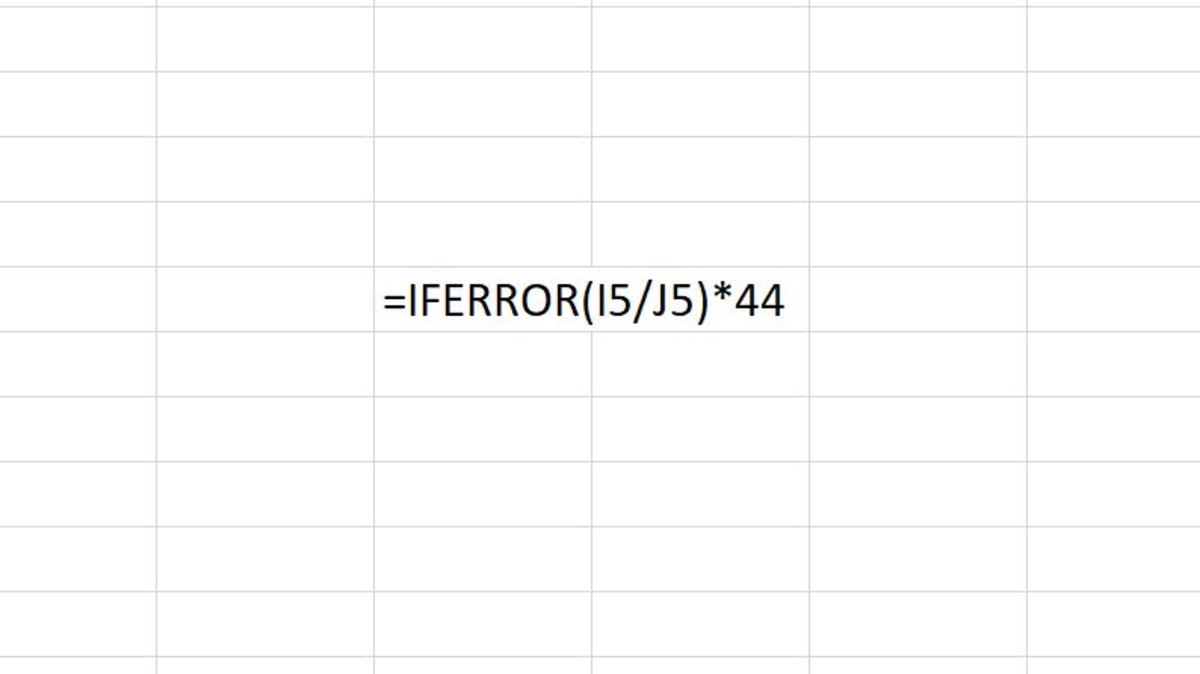 1200×674 remove errors excel iferror function turbofuture from turbofuture.com
  649×437 iferror function excel efinancialmodels from www.efinancialmodels.com
 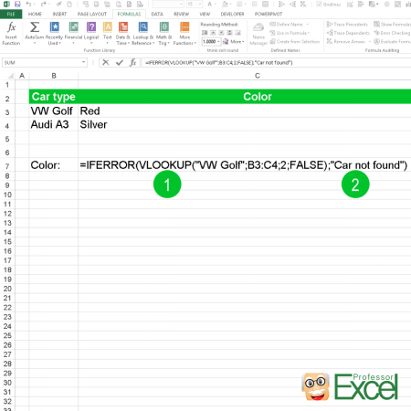 450×450 iferror handle error messages excel from professor-excel.com
 How To Use Iferror Function To Handle Errors In Excel Formulas was posted in February 12, 2026 at 7:41 am. If you wanna have it as yours, please click the Pictures and you will go to click right mouse then Save Image As and Click Save and download the How To Use Iferror Function To Handle Errors In Excel Formulas Picture.. Don’t forget to share this picture with others via Facebook, Twitter, Pinterest or other social medias! we do hope you'll get inspired by ExcelKayra... Thanks again! If you have any DMCA issues on this post, please contact us!