Vlookup Approximate Match Tutorial For Excel Beginners
Vlookup Approximate Match Tutorial For Excel Beginners - There are a lot of affordable templates out there, but it can be easy to feel like a lot of the best cost a amount of money, require best special design template. Making the best template format choice is way to your template success. And if at this time you are looking for information and ideas regarding the Vlookup Approximate Match Tutorial For Excel Beginners then, you are in the perfect place. Get this Vlookup Approximate Match Tutorial For Excel Beginners for free here. We hope this post Vlookup Approximate Match Tutorial For Excel Beginners inspired you and help you what you are looking for.
VLOOKUP Approximate Match: A Beginner’s Guide
VLOOKUP is a powerful Excel function that allows you to search for specific data within a range and return corresponding information from another column in that range. While many people are familiar with using VLOOKUP for exact matches, its “approximate match” capability opens up a whole new world of possibilities. This tutorial will guide you through the basics of VLOOKUP with approximate match, explaining how it works and providing practical examples for beginners.
Understanding VLOOKUP Basics
Before diving into approximate match, let’s briefly review the fundamental syntax of the VLOOKUP function:
=VLOOKUP(lookup_value, table_array, col_index_num, [range_lookup])- lookup_value: This is the value you want to search for in the first column of your data table.
- table_array: This is the range of cells containing your data table. The lookup value must be in the first column of this range.
- col_index_num: This is the column number within your table_array from which you want to retrieve the matching value. The first column is 1, the second is 2, and so on.
- [range_lookup]: This is an optional argument that determines whether VLOOKUP performs an exact or approximate match. It can be TRUE, FALSE, or omitted (omitted defaults to TRUE).
- TRUE (or omitted): Performs an approximate match. This is what we’ll focus on in this tutorial.
- FALSE: Performs an exact match. VLOOKUP returns #N/A if an exact match is not found.
The Power of Approximate Match
The beauty of approximate match lies in its ability to find the closest match when an exact match isn’t available. This is especially useful when dealing with numerical ranges, categories, or tiered systems. However, there’s a very important caveat: the first column of your `table_array` must be sorted in ascending order for approximate match to work correctly.
Here’s how it works:
- VLOOKUP searches for the `lookup_value` in the first column of the `table_array`.
- If it finds an exact match, it returns the corresponding value from the column specified by `col_index_num`.
- If it doesn’t find an exact match:
- VLOOKUP searches for the largest value in the first column that is less than or equal to the `lookup_value`.
- It then returns the corresponding value from the column specified by `col_index_num` on the same row as that largest value.
- If the `lookup_value` is smaller than the smallest value in the first column, VLOOKUP returns #N/A.
Example 1: Sales Commission Tiers
Let’s say you have a sales commission structure where commission rates vary based on sales volume. You have the following table:
| Sales Volume | Commission Rate |
|---|---|
| 0 | 0% |
| 10000 | 5% |
| 25000 | 7.5% |
| 50000 | 10% |
| 100000 | 12% |
Notice that the Sales Volume column is sorted in ascending order. Now, suppose a salesperson has achieved a sales volume of $35,000. You want to use VLOOKUP to determine their commission rate.
Here’s the VLOOKUP formula you would use:
=VLOOKUP(35000, A2:B6, 2, TRUE)Let’s break down the formula:
- lookup_value: 35000 (the salesperson’s sales volume)
- table_array: A2:B6 (the range containing the sales volume and commission rate data)
- col_index_num: 2 (the column containing the commission rate)
- range_lookup: TRUE (indicating an approximate match)
Here’s how VLOOKUP calculates the result:
- VLOOKUP doesn’t find an exact match for 35000 in the Sales Volume column.
- It finds the largest value in the Sales Volume column that is less than or equal to 35000, which is 25000.
- It returns the corresponding Commission Rate from the second column (column B) in the same row as 25000, which is 7.5%.
Therefore, the formula returns 7.5%, indicating that the salesperson’s commission rate is 7.5%.
Example 2: Letter Grades
Another common use case for VLOOKUP approximate match is assigning letter grades based on numerical scores. Consider this grading scale:
| Score | Grade |
|---|---|
| 0 | F |
| 60 | D |
| 70 | C |
| 80 | B |
| 90 | A |
If a student has a score of 75, you can use VLOOKUP to find their grade.
The formula would be:
=VLOOKUP(75, D2:E6, 2, TRUE)Breaking it down:
- lookup_value: 75 (the student’s score)
- table_array: D2:E6 (the range containing the score and grade data)
- col_index_num: 2 (the column containing the grade)
- range_lookup: TRUE (approximate match)
VLOOKUP works as follows:
- No exact match for 75 is found.
- The largest value in the Score column that’s less than or equal to 75 is 70.
- The corresponding Grade in column E is C.
The formula returns “C,” which is the correct grade for a score of 75.
Important Considerations
- Sorted First Column: This is absolutely crucial. The first column of your `table_array` must be sorted in ascending order for approximate match to work as expected. If it’s not sorted, VLOOKUP may return incorrect results or errors.
- #N/A Errors: As mentioned earlier, if the `lookup_value` is smaller than the smallest value in the first column, VLOOKUP will return #N/A. You can handle this error using the IFERROR function. For example: `=IFERROR(VLOOKUP(value, range, column, TRUE), “Below Minimum”)` would return “Below Minimum” if the lookup value is too small.
- Data Types: Ensure the data types in the `lookup_value` and the first column of your `table_array` are compatible. For example, if you’re looking up a number, make sure the values in the first column are also numbers, not text.
Beyond the Basics
While these examples illustrate the core concept, VLOOKUP approximate match can be combined with other Excel functions to create more sophisticated solutions. For instance, you can use it within nested formulas or with conditional formatting to highlight specific data points.
Conclusion
VLOOKUP approximate match is a valuable tool for handling situations where exact matches aren’t required or aren’t possible. By understanding its mechanics and adhering to the rule of sorting the first column, you can leverage its power to perform lookups based on ranges, categories, and tiered systems. Practice with different scenarios to master this useful Excel function and enhance your data analysis capabilities.
 768×334 vlookup approximate match myexcelonline from www.myexcelonline.com
  1280×720 excel tutorial troubleshoot vlookup approximate match from exceljet.net
 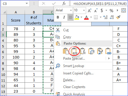 452×338 vlookup approximate match excelnotes from excelnotes.com
  1187×477 vlookup exact approximate match excel from www.extendoffice.com
  1280×720 vlookup approximate match microsoft excel basic advanced from www.goskills.com
  680×331 mastering vlookup excel step step guide from www.simplilearn.com
  405×297 excel vlookup tutorial beginners formula examples from ablebits.com
  1280×600 exact approximate matching vlookup excel from ms-office.wonderhowto.com
 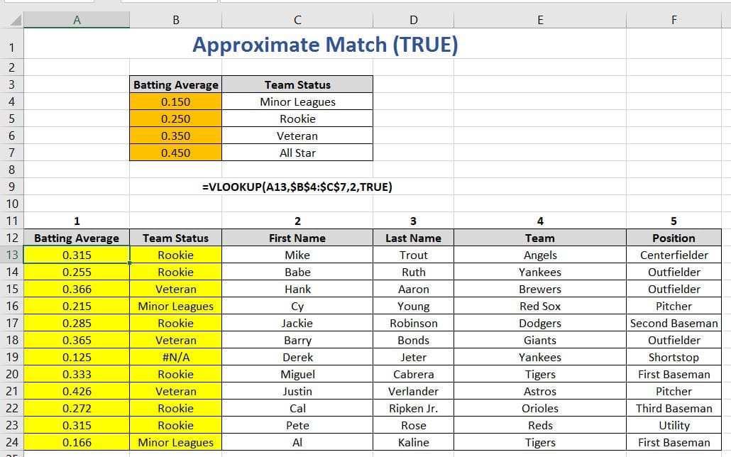 1030×644 vlookup function excel excelbuddycom from excelbuddy.com
 Vlookup Approximate Match Tutorial For Excel Beginners was posted in January 11, 2026 at 7:07 am. If you wanna have it as yours, please click the Pictures and you will go to click right mouse then Save Image As and Click Save and download the Vlookup Approximate Match Tutorial For Excel Beginners Picture.. Don’t forget to share this picture with others via Facebook, Twitter, Pinterest or other social medias! we do hope you'll get inspired by ExcelKayra... Thanks again! If you have any DMCA issues on this post, please contact us!