Create Gantt Chart In Excel Without Using Add-ins
Create Gantt Chart In Excel Without Using Add-ins - There are a lot of affordable templates out there, but it can be easy to feel like a lot of the best cost a amount of money, require best special design template. Making the best template format choice is way to your template success. And if at this time you are looking for information and ideas regarding the Create Gantt Chart In Excel Without Using Add-ins then, you are in the perfect place. Get this Create Gantt Chart In Excel Without Using Add-ins for free here. We hope this post Create Gantt Chart In Excel Without Using Add-ins inspired you and help you what you are looking for.
Creating a Gantt chart in Excel without relying on add-ins is a surprisingly straightforward and effective way to visualize project timelines and track progress. While dedicated project management software offers more advanced features, Excel provides a readily accessible and customizable solution for basic Gantt chart needs. This guide outlines the steps to create a functional Gantt chart using Excel’s built-in features, focusing on conditional formatting and stacked bar charts.
Setting Up the Data
The foundation of any Gantt chart is well-organized data. Start by creating a table with the following columns:
- Task: A descriptive name for each task in your project.
- Start Date: The date the task is scheduled to begin.
- Duration (Days): The number of days the task is expected to take.
- End Date: (Optional, but recommended) A calculated field showing the expected completion date of the task. This can be calculated using the formula: `=Start Date + Duration`.
Populate this table with the tasks, start dates, and durations specific to your project. Accurate and detailed data is crucial for a useful and informative Gantt chart.
Creating the Stacked Bar Chart
The core of the Gantt chart visualization is a stacked bar chart. Here’s how to create one:
- Select Data:** Select the `Task` and `Start Date` columns. Hold down the Ctrl key (or Cmd key on Mac) and select the `Duration (Days)` column. This will select non-contiguous columns.
- Insert Chart:** Go to the `Insert` tab on the Excel ribbon. In the `Charts` group, click on the `Insert Bar Chart` dropdown menu.
- Choose Stacked Bar:** Select the `Stacked Bar` chart option (the second option in the 2D-Bar section).
Excel will generate a basic stacked bar chart. You’ll notice that the chart displays the tasks on the vertical axis and the start dates and durations as bars on the horizontal axis. However, it needs significant adjustments to resemble a proper Gantt chart.
Formatting the Chart
This is where the magic happens. You’ll need to adjust the chart’s appearance to clearly display the project timeline:
- Invert Axis Order:** The tasks are displayed in reverse order. To fix this, right-click on the vertical axis (task names) and choose `Format Axis`. In the `Format Axis` pane, under `Axis Options`, check the box labeled `Categories in reverse order`. Close the Format Axis pane.
- Hide the Start Date Bars:** The “Start Date” series is represented by bars. These bars should be invisible, as they only serve to position the “Duration” bars correctly. Click on any of the “Start Date” bars in the chart. This selects the entire “Start Date” series. Right-click and choose `Format Data Series`. In the `Format Data Series` pane, go to the `Fill & Line` tab (the paint bucket icon). Under `Fill`, select `No fill`. Under `Border`, select `No line`. Close the Format Data Series pane. The “Start Date” bars should now be invisible, leaving only the “Duration” bars visible.
- Adjust the Horizontal Axis:** The horizontal axis (dates) needs to be adjusted to display the entire project timeline appropriately. Right-click on the horizontal axis and choose `Format Axis`. In the `Format Axis` pane, under `Axis Options`, you’ll find the `Bounds` section.
- Minimum:** Set the `Minimum` value to a date before the earliest `Start Date` in your data. Excel uses a serial number to represent dates, so you’ll need to convert the desired date to its serial number. You can do this by typing the date into a cell in your spreadsheet, formatting the cell as `General`, and noting the resulting number. Use this number as the `Minimum` value. Alternatively, use the formula `=DATE(YYYY,MM,DD)` in a cell, where YYYY is the year, MM is the month, and DD is the day. For instance, `=DATE(2024,1,1)` represents January 1, 2024. After entering the formula, format the cell as `General` to see the serial number.
- Maximum:** Set the `Maximum` value to a date after the latest `End Date` in your data, using the same method to find the serial number.
- Units:** Adjust the `Major unit` to something appropriate for your timeline (e.g., 7 for weekly increments, 30 or 31 for monthly increments). This will determine the spacing of the gridlines.
Close the Format Axis pane.
- Customize Colors:** You can customize the colors of the “Duration” bars to represent different task categories or project phases. Click on a “Duration” bar to select the series, then right-click and choose `Format Data Series`. In the `Fill & Line` tab, select a desired color under `Fill`. You can apply different colors to individual bars by clicking on a bar twice (slowly – not a double-click) to select just that bar, and then changing its fill color.
Adding Labels and Fine-Tuning
To further enhance the Gantt chart, consider adding labels and making further refinements:
- Add Data Labels:** While not always necessary, adding data labels to the “Duration” bars can show the duration in days. Click on the “Duration” bars, then right-click and choose `Add Data Labels`. You may need to format the data labels to position them appropriately (e.g., inside end).
- Adjust Chart Title:** Edit the chart title to accurately reflect the project being visualized.
- Format Gridlines:** You can change the appearance of the gridlines (e.g., color, line style) by right-clicking on a gridline and choosing `Format Gridlines`.
- Conditional Formatting (for Progress):** To visualize task progress, you can add another column to your data table called “% Complete”. Then, using conditional formatting, you could color the bars based on their completion percentage. Select the range of cells containing the durations. Then, go to “Home” -> “Conditional Formatting” -> “Data Bars”. Choose a gradient or solid fill that you like. Then, go to “Home” -> “Conditional Formatting” -> “Manage Rules”. Edit the rule. Set “Minimum” to “Number” with value 0, and “Maximum” to “Number” with value 1. Then, check “Show Bar Only”. This shows progress inside the Duration Bar itself.
By following these steps, you can create a functional and visually appealing Gantt chart in Excel without any add-ins. Remember that this approach is best suited for relatively simple projects. For more complex projects with dependencies, resource allocation, and critical path analysis, dedicated project management software is recommended.
 493×579 create gantt chart microsoft excel from www.thewindowsclub.com
  624×380 create gantt chart excel easily teachexcelcom from www.teachexcel.com
  723×643 create gantt chart excel from www.extendoffice.com
 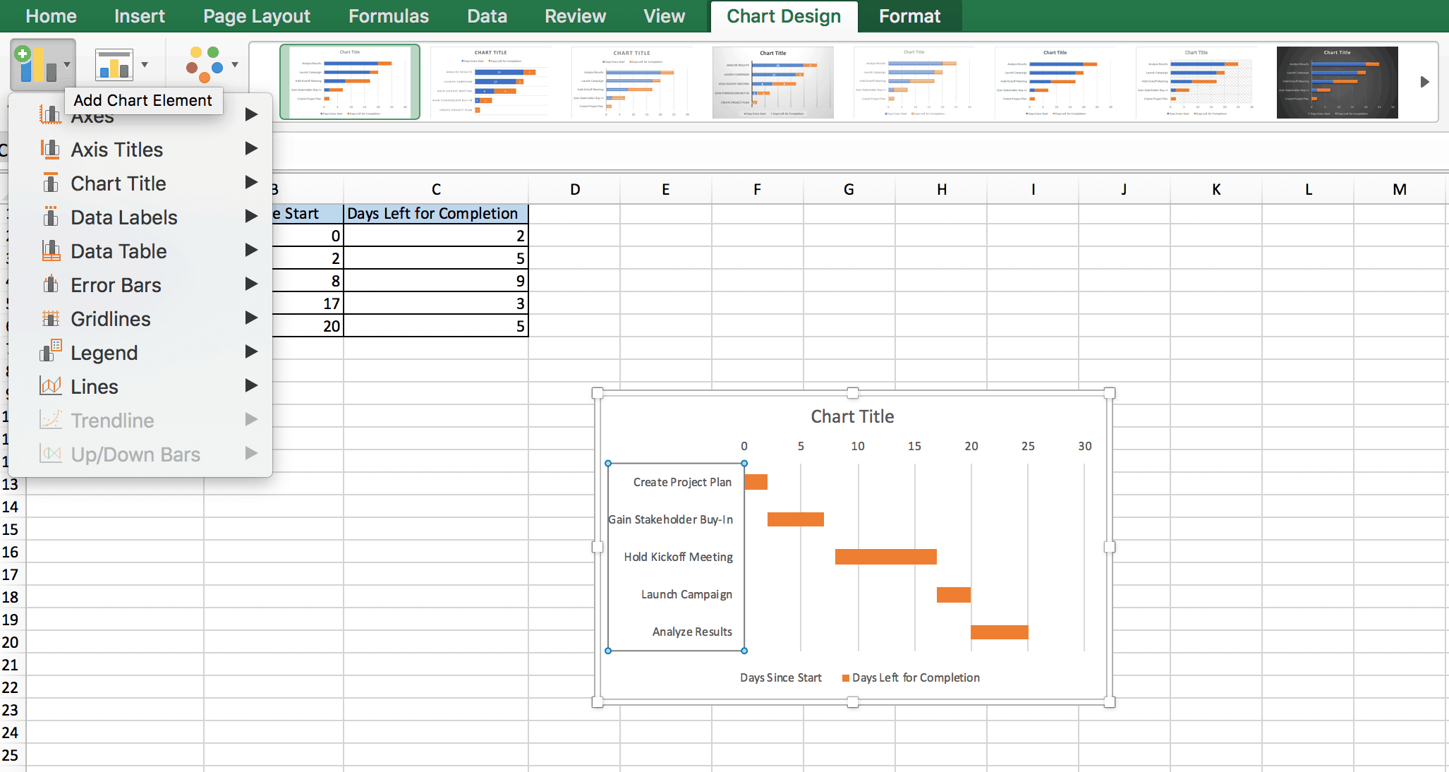 2054×1094 gantt charts excel templates tutorial video smartsheet from smartsheet.com
  502×406 gantt chart excelnotes from excelnotes.com
  1295×733 gantt chart excel developer publish from developerpublish.com
  1614×1122 gantt chart excel lucidchart from www.lucidchart.com
 Create Gantt Chart In Excel Without Using Add-ins was posted in October 6, 2025 at 5:55 pm. If you wanna have it as yours, please click the Pictures and you will go to click right mouse then Save Image As and Click Save and download the Create Gantt Chart In Excel Without Using Add-ins Picture.. Don’t forget to share this picture with others via Facebook, Twitter, Pinterest or other social medias! we do hope you'll get inspired by ExcelKayra... Thanks again! If you have any DMCA issues on this post, please contact us!