How To Calculate Compound Interest In Excel Step By Step
How To Calculate Compound Interest In Excel Step By Step - There are a lot of affordable templates out there, but it can be easy to feel like a lot of the best cost a amount of money, require best special design template. Making the best template format choice is way to your template success. And if at this time you are looking for information and ideas regarding the How To Calculate Compound Interest In Excel Step By Step then, you are in the perfect place. Get this How To Calculate Compound Interest In Excel Step By Step for free here. We hope this post How To Calculate Compound Interest In Excel Step By Step inspired you and help you what you are looking for.
Calculating compound interest in Excel is a straightforward process that can be accomplished using a simple formula. Compound interest, unlike simple interest, takes into account the interest earned on the principal amount as well as the accumulated interest from previous periods. This means that your money grows at an accelerating rate over time. Understanding how to calculate this in Excel allows you to forecast investment growth, plan for future savings goals, or analyze loan repayments.
Here’s a step-by-step guide on how to calculate compound interest in Excel:
-
Open a New Excel Worksheet: Begin by opening Microsoft Excel and creating a new, blank worksheet. This will be your canvas for performing the calculations and organizing the data.
-
Label Your Columns: To keep your calculations organized and easy to understand, it’s best to label your columns. Create the following column headers in the first row:
- Principal (P): This column will hold the initial amount of money you’re investing or borrowing.
- Interest Rate (r): This column will contain the annual interest rate expressed as a decimal (e.g., 5% would be 0.05).
- Number of Times Compounded per Year (n): This column indicates how many times the interest is compounded within a year (e.g., monthly compounding would be 12, quarterly would be 4, annually would be 1).
- Number of Years (t): This column represents the total number of years the money will be invested or borrowed.
- Future Value (FV): This column will hold the result of the compound interest calculation, which is the total amount you’ll have at the end of the investment period.
-
Enter Your Data: Now, populate the first four columns (Principal, Interest Rate, Number of Times Compounded per Year, and Number of Years) with the specific values you want to use in your calculation. For example:
- Principal (P): $10,000
- Interest Rate (r): 0.05 (5%)
- Number of Times Compounded per Year (n): 12 (monthly)
- Number of Years (t): 5
-
Enter the Compound Interest Formula: This is the core step. In the “Future Value (FV)” column (next to the row containing your data), enter the following Excel formula:
=P*(1+r/n)^(n*t)Replace `P`, `r`, `n`, and `t` with the cell references corresponding to the values you entered in the previous step. For example, if your principal is in cell A2, your interest rate is in cell B2, your compounding frequency is in cell C2, and your number of years is in cell D2, the formula would be:
=A2*(1+B2/C2)^(C2*D2)Let’s break down this formula:
- A2: Represents the principal amount.
- B2: Represents the annual interest rate.
- C2: Represents the number of times the interest is compounded per year.
- D2: Represents the number of years.
- (1+B2/C2): This calculates the interest rate per compounding period. It divides the annual interest rate by the number of compounding periods per year and adds 1.
- ^(C2*D2): This raises the previous result to the power of the total number of compounding periods (number of compounding periods per year multiplied by the number of years).
- A2*…: Finally, the principal amount is multiplied by the result of the exponentiation to calculate the future value.
-
Press Enter: After entering the formula, press Enter. The cell in the “Future Value (FV)” column will now display the calculated future value of your investment, taking into account compound interest.
-
Format the Result: To display the future value as currency, select the cell containing the result and click the “Currency” format option in the “Number” group on the “Home” tab. This will add a dollar sign and display the value with two decimal places.
-
Experiment with Different Values: One of the benefits of using Excel is the ability to easily change the input values and see how they affect the outcome. You can change the principal, interest rate, compounding frequency, or number of years to explore different investment scenarios. Each time you change a value, the future value will automatically update.
-
Calculate for Multiple Scenarios: You can create multiple rows of data to compare different investment options. Simply enter the data for each scenario in its own row and copy the formula from the first row down to the other rows. Excel will automatically adjust the cell references in the formula to match each row.
-
Additions and Contributions (Optional): If you’re making regular contributions to your investment, the formula becomes more complex. Excel doesn’t have a single, straightforward function for calculating compound interest with regular contributions. You’ll typically need to use a combination of formulas, including the `FV` function (Future Value) or create a custom calculation using a loop-like structure with multiple rows representing each period.
The `FV` function simplifies the calculation of future value with regular payments. The syntax is:
=FV(rate, nper, pmt, [pv], [type])- rate: The interest rate per period (annual rate / number of periods per year).
- nper: The total number of payment periods (number of years * number of periods per year).
- pmt: The payment made each period. Enter this as a negative number if you are paying into the investment.
- pv: (Optional) The present value or initial investment. If omitted, it is assumed to be 0.
- type: (Optional) Indicates when payments are due. 0 indicates payments are due at the end of the period (default), and 1 indicates payments are due at the beginning of the period.
For example, if you invest $1000 initially, add $100 each month for 5 years at an annual interest rate of 5%, the formula would be:
=FV(0.05/12, 5*12, -100, -1000, 0)This formula calculates the future value considering the initial investment and the regular monthly contributions.
By following these steps, you can effectively calculate compound interest in Excel and gain valuable insights into the potential growth of your investments. Remember to pay attention to the compounding frequency, as it significantly impacts the final outcome.
 1163×532 calculate compound interest excel quickexcel from quickexcel.com
  693×452 calculate compound interest excel calculate from www.educba.com
  1280×720 calculate compound interest excel techyuga from www.techyuga.com
  419×222 compound interest function excel from www.exceltip.com
 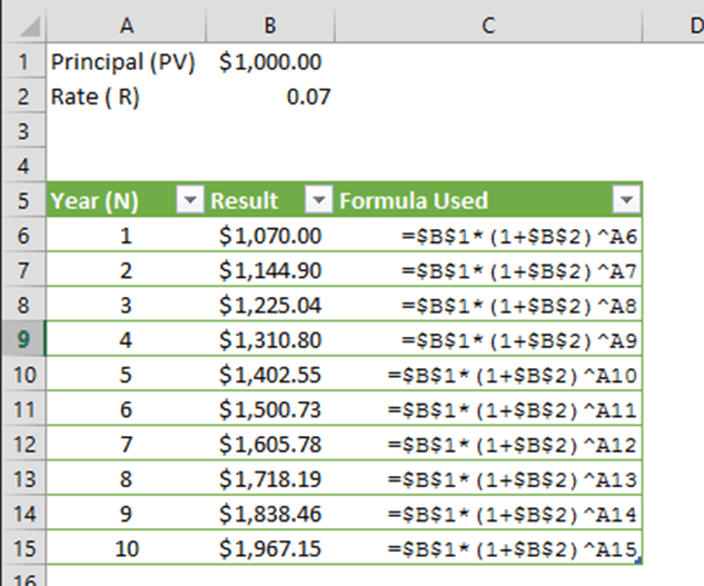 633×527 calculate compound interest excel from officepowerups.com
 How To Calculate Compound Interest In Excel Step By Step was posted in December 9, 2025 at 3:45 pm. If you wanna have it as yours, please click the Pictures and you will go to click right mouse then Save Image As and Click Save and download the How To Calculate Compound Interest In Excel Step By Step Picture.. Don’t forget to share this picture with others via Facebook, Twitter, Pinterest or other social medias! we do hope you'll get inspired by ExcelKayra... Thanks again! If you have any DMCA issues on this post, please contact us!