How To Calculate Depreciation Using Straight-line Method In Excel
How To Calculate Depreciation Using Straight-line Method In Excel - There are a lot of affordable templates out there, but it can be easy to feel like a lot of the best cost a amount of money, require best special design template. Making the best template format choice is way to your template success. And if at this time you are looking for information and ideas regarding the How To Calculate Depreciation Using Straight-line Method In Excel then, you are in the perfect place. Get this How To Calculate Depreciation Using Straight-line Method In Excel for free here. We hope this post How To Calculate Depreciation Using Straight-line Method In Excel inspired you and help you what you are looking for.
Calculating Straight-Line Depreciation in Excel
Depreciation is an accounting method used to allocate the cost of a tangible asset over its useful life. The straight-line method is one of the simplest and most commonly used depreciation methods. It allocates an equal amount of depreciation expense to each period of the asset’s useful life. Excel provides built-in functions to easily calculate straight-line depreciation.
Understanding the Straight-Line Method
The straight-line method calculates depreciation based on the following formula:
Depreciation Expense = (Cost – Salvage Value) / Useful Life
Where:
- Cost: The original cost of the asset.
- Salvage Value: The estimated value of the asset at the end of its useful life (also known as residual value).
- Useful Life: The estimated number of periods (years, months, etc.) that the asset will be used.
This formula determines the annual depreciation expense. To calculate the monthly depreciation expense, you would divide the annual depreciation expense by 12.
Using the SLN Function in Excel
Excel provides the `SLN` function to calculate straight-line depreciation. The syntax for the `SLN` function is:
=SLN(cost, salvage, life)
Where:
- cost: The original cost of the asset.
- salvage: The estimated salvage value of the asset.
- life: The estimated useful life of the asset (in the same time units as the period you want the depreciation for – e.g., years for annual depreciation, months for monthly depreciation).
Example 1: Calculating Annual Depreciation
Let’s say a company purchases a machine for $50,000. The estimated salvage value is $5,000, and the useful life is 10 years. To calculate the annual depreciation expense using the `SLN` function:
- Open an Excel spreadsheet.
- In cell A1, enter “Cost”.
- In cell A2, enter “$50000”.
- In cell B1, enter “Salvage Value”.
- In cell B2, enter “$5000”.
- In cell C1, enter “Useful Life (Years)”.
- In cell C2, enter “10”.
- In cell D1, enter “Annual Depreciation”.
- In cell D2, enter the following formula: `=SLN(A2, B2, C2)`.
- The result in cell D2 will be $4,500, which is the annual depreciation expense.
Excel automatically calculates `($50,000 – $5,000) / 10 = $4,500`.
Example 2: Calculating Monthly Depreciation
Using the same example as above, let’s calculate the monthly depreciation expense. The key is to express the useful life in months.
- Open an Excel spreadsheet (or continue with the previous one).
- In cell A1, enter “Cost”.
- In cell A2, enter “$50000”.
- In cell B1, enter “Salvage Value”.
- In cell B2, enter “$5000”.
- In cell C1, enter “Useful Life (Months)”.
- In cell C2, enter “120” (10 years * 12 months/year).
- In cell D1, enter “Monthly Depreciation”.
- In cell D2, enter the following formula: `=SLN(A2, B2, C2)`.
- The result in cell D2 will be $375, which is the monthly depreciation expense.
Excel calculates `($50,000 – $5,000) / 120 = $375`.
Creating a Depreciation Schedule in Excel
A depreciation schedule is a table that shows the depreciation expense, accumulated depreciation, and book value of an asset over its useful life. Here’s how to create a basic straight-line depreciation schedule in Excel:
- Set up the headings:
- In cell A1, enter “Year”.
- In cell B1, enter “Depreciation Expense”.
- In cell C1, enter “Accumulated Depreciation”.
- In cell D1, enter “Book Value”.
- Enter the years:
- In cell A2, enter “1”.
- In cell A3, enter “2”.
- Select cells A2 and A3, then drag the fill handle (the small square at the bottom right of the selected cells) down to cell A11 to auto-fill the years 3 through 10.
- Calculate the depreciation expense:
- Assuming the cost, salvage value, and useful life are in cells E2, E3, and E4 respectively, enter the following formula in cell B2: `=SLN(E2, E3, E4)`. (You can also directly enter the values instead of cell references: `=SLN(50000,5000,10)` if you don’t want to create the cells with those values).
- Copy the formula in cell B2 down to cells B3 through B11. Since we are using fixed references we need to lock these cells. Change your formula to `SLN($E$2, $E$3, $E$4)` and copy it down.
- Calculate the accumulated depreciation:
- In cell C2, enter `=B2`. This is the accumulated depreciation for the first year, which is equal to the depreciation expense for that year.
- In cell C3, enter `=C2+B3`. This adds the depreciation expense for the current year to the accumulated depreciation from the previous year.
- Copy the formula in cell C3 down to cells C4 through C11.
- Calculate the book value:
- In cell D2, enter `=E2-C2`. E2 holds the initial cost from our previous setup.
- In cell D3, enter `=E2-C3`. This subtracts the accumulated depreciation from the original cost of the asset.
- Copy the formula in cell D3 down to cells D4 through D11. Like before, fix the reference to E2 by changing the formula in D2 to `=$E$2-C2` and copy it down.
- Format the spreadsheet (optional):
- Format the cells containing monetary values (Cost, Salvage Value, Depreciation Expense, Accumulated Depreciation, Book Value) as currency.
- Adjust column widths for better readability.
- Add borders to the table.
Important Considerations
- Consistency: Once a depreciation method is chosen, it should be applied consistently throughout the asset’s useful life unless there is a valid reason to change it.
- Estimates: Salvage value and useful life are estimates. Review and adjust these estimates periodically as needed.
- Other Depreciation Methods: While the straight-line method is simple, other methods, such as the double-declining balance or sum-of-the-years’ digits methods, may be more appropriate for certain assets. These methods can also be calculated in Excel using functions like `DDB` and `SYD`.
- Tax Implications: Consult with a tax professional to understand the tax implications of depreciation and the allowable depreciation methods for your specific situation.
Conclusion
Calculating straight-line depreciation in Excel is straightforward using the `SLN` function. By understanding the formula and utilizing Excel’s capabilities, you can accurately track the depreciation of your assets and create informative depreciation schedules.
 700×400 easily calculate straight depreciation excel exceldatapro from exceldatapro.com
  895×512 straight depreciation calculator from myexceltemplates.com
  800×348 straight depreciation definition formula accounting from exceldatapro.com
 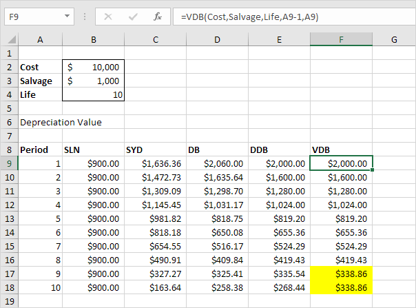 604×447 depreciation formulas excel complete tutorial from www.excel-easy.com
  634×643 straight depreciation schedule calculator double entry bookkeeping from www.double-entry-bookkeeping.com
  768×395 straight depreciation formula calculator excel template from www.educba.com
 How To Calculate Depreciation Using Straight-line Method In Excel was posted in November 5, 2025 at 12:11 pm. If you wanna have it as yours, please click the Pictures and you will go to click right mouse then Save Image As and Click Save and download the How To Calculate Depreciation Using Straight-line Method In Excel Picture.. Don’t forget to share this picture with others via Facebook, Twitter, Pinterest or other social medias! we do hope you'll get inspired by ExcelKayra... Thanks again! If you have any DMCA issues on this post, please contact us!