Home » Excel Templates » How To Calculate Monthly Payments For Loans In Excel

How To Calculate Monthly Payments For Loans In Excel

Tuesday, August 26th 2025. | Excel Templates

How To Calculate Monthly Payments For Loans In Excel - There are a lot of affordable templates out there, but it can be easy to feel like a lot of the best cost a amount of money, require best special design template. Making the best template format choice is way to your template success. And if at this time you are looking for information and ideas regarding the How To Calculate Monthly Payments For Loans In Excel then, you are in the perfect place. Get this How To Calculate Monthly Payments For Loans In Excel for free here. We hope this post How To Calculate Monthly Payments For Loans In Excel inspired you and help you what you are looking for.

calculate monthly payment excel steps

Here’s an explanation of how to calculate monthly loan payments in Excel, formatted in HTML, covering various scenarios and useful functions.

Calculating Loan Payments in Excel

Excel provides powerful functions to easily calculate loan payments, empowering you to understand your financial obligations for mortgages, car loans, personal loans, and more. The core function we’ll be using is PMT, but we’ll also explore related functions like IPMT and PPMT to break down the payment into its interest and principal components.

The PMT Function: Your Primary Tool

The PMT function is the cornerstone for calculating loan payments. Its syntax is as follows:

=PMT(rate, nper, pv, [fv], [type])

Let’s break down each argument:

rate: The interest rate *per period*. This is crucial! If you have an annual interest rate, you’ll need to divide it by the number of payment periods per year (usually 12 for monthly payments). For example, if the annual rate is 6%, the monthly rate would be 0.06/12 = 0.005.
nper: The total number of payment periods. For a 30-year mortgage with monthly payments, this would be 30 * 12 = 360.
pv: The present value, or the loan amount. This is the amount you’re borrowing.
[fv]: (Optional) The future value, or the cash balance you want to attain after the last payment is made. If omitted, it’s assumed to be 0 (the typical loan scenario).
[type]: (Optional) When payments are due. 0 (or omitted) indicates payments are due at the end of the period (ordinary annuity), and 1 indicates payments are due at the beginning of the period (annuity due). Mortgages and most loans are ordinary annuities.

Example: Calculating a Simple Loan Payment

Let’s say you want to borrow $20,000 at an annual interest rate of 5% for 5 years, with monthly payments. Here’s how you would calculate the monthly payment in Excel:

Open an Excel spreadsheet.
In cell A1, enter “Loan Amount:”.
In cell B1, enter 20000.
In cell A2, enter “Annual Interest Rate:”.
In cell B2, enter 0.05 (representing 5%).
In cell A3, enter “Loan Term (Years):”.
In cell B3, enter 5.
In cell A4, enter “Monthly Payment:”.
In cell B4, enter the following formula: =PMT(B2/12, B3*12, B1)

Excel will calculate the monthly payment, which will be a negative number (representing cash outflow). You might want to put a minus sign in front of the formula to display it as a positive value: =-PMT(B2/12, B3*12, B1)

Understanding Interest and Principal Components with IPMT and PPMT

While PMT gives you the total monthly payment, you might want to know how much of each payment goes towards interest and how much goes towards the principal. This is where IPMT and PPMT come in handy.

The IPMT Function: Interest Payment

The IPMT function calculates the interest portion of a loan payment for a specific period. Its syntax is:

=IPMT(rate, per, nper, pv, [fv], [type])

rate: Same as in PMT (interest rate per period).
per: The period for which you want to find the interest payment. For example, if you want to know the interest portion of the first month’s payment, per would be 1. For the second month, it would be 2, and so on.
nper: Same as in PMT (total number of payment periods).
pv: Same as in PMT (present value, or loan amount).
[fv]: (Optional) Same as in PMT (future value).
[type]: (Optional) Same as in PMT (payment due at the beginning or end of the period).

The PPMT Function: Principal Payment

The PPMT function calculates the principal portion of a loan payment for a specific period. Its syntax is almost identical to IPMT:

=PPMT(rate, per, nper, pv, [fv], [type])

The arguments are the same as for IPMT.

Example: Breaking Down a Monthly Payment

Using the same loan details as before ($20,000 at 5% for 5 years with monthly payments), let’s calculate the interest and principal components of the first month’s payment:

Continuing from the previous example, in cell A5, enter “Interest (Month 1):”.
In cell B5, enter the following formula: =IPMT(B2/12, 1, B3*12, B1)
In cell A6, enter “Principal (Month 1):”.
In cell B6, enter the following formula: =PPMT(B2/12, 1, B3*12, B1)

Excel will calculate the interest and principal portions of the first month’s payment. Again, these will be negative values. You might want to add a minus sign in front of the formulas.

Important: For any given period, PMT should equal the sum of IPMT and PPMT for that period (within rounding errors).

Creating an Amortization Schedule

An amortization schedule is a table that shows the breakdown of each loan payment into interest and principal over the life of the loan. Here’s how you can create one in Excel:

Set up your loan parameters (loan amount, interest rate, loan term) as in the previous examples (cells B1, B2, B3).
In row 8, create the following column headers: “Period”, “Beginning Balance”, “Payment”, “Interest”, “Principal”, “Ending Balance”.
In cell A9, enter 1 (the first period).
In cell B9, enter =B1 (the initial loan amount).
In cell C9, enter =-PMT(B2/12, B3*12, B1) (the total monthly payment, locked).
In cell D9, enter =-IPMT(B2/12, A9, B3*12, B1) (the interest portion).
In cell E9, enter =-PPMT(B2/12, A9, B3*12, B1) (the principal portion).
In cell F9, enter =B9-E9 (the ending balance after the first payment).
In cell A10, enter =A9+1 (the next period).
In cell B10, enter =F9 (the beginning balance for this period is the ending balance from the previous period).
Copy cells C9, D9, E9, and F9 down to row 10.
Select rows 10 and drag the fill handle (the small square at the bottom right corner of the selection) down to row 368 (for a 30-year mortgage – 360 months + 8 header rows). You may need to adjust this for other loan lengths.

Your amortization schedule is now complete. You can format the columns as currency for better readability.

Key Observations in an Amortization Schedule:

The “Interest” portion of the payment decreases over time, while the “Principal” portion increases.
The “Ending Balance” gradually decreases towards zero. The final ending balance may not be exactly zero due to rounding, but it should be very close.

Dealing with Different Payment Frequencies

The examples above assume monthly payments. If your loan has a different payment frequency (e.g., bi-weekly), you’ll need to adjust the rate and nper accordingly.

For example, with bi-weekly payments (26 payments per year):

rate: Annual interest rate / 26
nper: Loan term in years * 26

Error Handling and Considerations

Interest Rate Units: Always ensure your interest rate is expressed as a decimal (e.g., 5% = 0.05).
Division by Zero: Avoid division by zero errors. Ensure the annual interest rate and the loan term are not zero.
Negative Loan Amount: While you can technically use a negative loan amount (pv), it’s generally clearer to use a positive value and adjust the final result (by adding a minus sign to the formula) if you want the payment to be displayed as a positive number.
Rounding Errors: Be aware that Excel calculations may involve slight rounding errors, especially when dealing with large loan amounts or long loan terms. This is usually insignificant.

By understanding and applying these Excel functions and principles, you can effectively calculate and analyze loan payments, build amortization schedules, and make informed financial decisions.

800×600 calculate monthly payment excel steps from www.wikihow.com

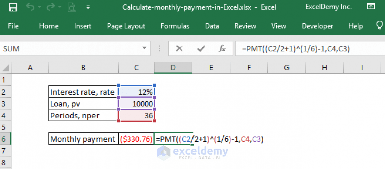766×336 calculate monthly payment excel excel calculator from www.exceldemy.com

535×400 calculating loan payments excel pmt function dummies from www.dummies.com

How To Calculate Monthly Payments For Loans In Excel was posted in August 26, 2025 at 6:56 pm. If you wanna have it as yours, please click the Pictures and you will go to click right mouse then Save Image As and Click Save and download the How To Calculate Monthly Payments For Loans In Excel Picture.. Don’t forget to share this picture with others via Facebook, Twitter, Pinterest or other social medias! we do hope you'll get inspired by ExcelKayra... Thanks again! If you have any DMCA issues on this post, please contact us!