How To Calculate ROI For Multiple Investments In Excel
How To Calculate ROI For Multiple Investments In Excel - There are a lot of affordable templates out there, but it can be easy to feel like a lot of the best cost a amount of money, require best special design template. Making the best template format choice is way to your template success. And if at this time you are looking for information and ideas regarding the How To Calculate ROI For Multiple Investments In Excel then, you are in the perfect place. Get this How To Calculate ROI For Multiple Investments In Excel for free here. We hope this post How To Calculate ROI For Multiple Investments In Excel inspired you and help you what you are looking for.
Okay, here’s an HTML formatted explanation of how to calculate Return on Investment (ROI) for multiple investments in Excel, aiming for approximately 1000 words.
Calculating Return on Investment (ROI) is crucial for evaluating the profitability and efficiency of your investments. When dealing with multiple investments, tracking and comparing their performance becomes even more important. Microsoft Excel provides powerful tools to streamline this process. This guide will walk you through calculating ROI for various investments in Excel, covering different scenarios and providing practical examples.
Understanding ROI
Before diving into Excel, let’s define ROI. ROI measures the gain or loss generated from an investment relative to the amount of money invested. The formula is:
ROI = (Net Profit / Cost of Investment) * 100
Where:
- Net Profit is the total gain from the investment minus the initial cost.
- Cost of Investment is the initial amount invested.
The result is expressed as a percentage, making it easy to compare the performance of different investments, regardless of their scale.
Setting Up Your Excel Spreadsheet
First, organize your data in a clear and structured manner within your Excel spreadsheet. A well-organized spreadsheet will make calculations easier and reduce the likelihood of errors. Consider the following columns:
- Investment Name/ID: A unique identifier for each investment (e.g., Stock A, Rental Property 1, Project X).
- Initial Investment Cost: The amount of money initially invested.
- Revenue/Gain: The total revenue or gain generated by the investment.
- Expenses: Any expenses associated with the investment (e.g., maintenance costs, management fees, taxes).
- Net Profit: Calculated as Revenue/Gain minus Expenses.
- ROI: Calculated using the ROI formula.
Here’s an example of how your spreadsheet might look:
| Investment Name/ID | Initial Investment Cost | Revenue/Gain | Expenses | Net Profit | ROI |
|---|---|---|---|---|---|
| Stock A | 10000 | 12000 | 500 | ||
| Rental Property 1 | 150000 | 20000 | 8000 | ||
| Project X | 5000 | 7000 | 1000 |
Calculating Net Profit in Excel
The first step is to calculate the Net Profit for each investment. In the “Net Profit” column, use the following formula:
=C2-D2 (Assuming Revenue/Gain is in column C and Expenses are in column D, starting from row 2)
Enter this formula in the first cell of the “Net Profit” column (E2 in this example). Then, drag the fill handle (the small square at the bottom-right corner of the cell) down to apply the formula to all rows.
Calculating ROI in Excel
Next, calculate the ROI for each investment using the ROI formula. In the “ROI” column, use the following formula:
=(E2/B2)*100 (Assuming Net Profit is in column E and Initial Investment Cost is in column B, starting from row 2)
Enter this formula in the first cell of the “ROI” column (F2 in this example). Drag the fill handle down to apply the formula to all rows. You’ll likely want to format this column as a percentage. Select the entire column, then click the “%” button in the “Number” group on the “Home” tab. You can also adjust the number of decimal places displayed using the increase/decrease decimal buttons next to the percentage button.
After applying the formulas, your table should look something like this:
| Investment Name/ID | Initial Investment Cost | Revenue/Gain | Expenses | Net Profit | ROI |
|---|---|---|---|---|---|
| Stock A | 10000 | 12000 | 500 | 11500 | 115% |
| Rental Property 1 | 150000 | 20000 | 8000 | 12000 | 8% |
| Project X | 5000 | 7000 | 1000 | 6000 | 120% |
Advanced ROI Calculations and Analysis
Beyond the basic ROI calculation, Excel offers features to enhance your analysis and make informed investment decisions.
1. Time-Adjusted ROI (Annualized ROI)
When comparing investments held for different periods, a simple ROI calculation can be misleading. To account for time, you can calculate the Annualized ROI. If your ROI is over a period longer than one year, you can annualize it. The formula is:
Annualized ROI = ((1 + ROI)^(1/n)) – 1
Where ‘n’ is the number of years the investment was held.
Add a column for “Years Held” and another for “Annualized ROI”. Let’s say “Years Held” is in column G and “Annualized ROI” will be in column H. In the first cell of the “Annualized ROI” column (H2), use the following formula:
=((1+F2)^(1/G2))-1 (Assuming ROI is in column F and Years Held in column G)
Format the “Annualized ROI” column as a percentage.
2. Weighted Average ROI
If you want to calculate the overall ROI of your entire investment portfolio, you can use a weighted average. This accounts for the different amounts invested in each asset.
- Calculate the proportion of each investment: Divide the initial investment cost of each investment by the total investment cost. Add a new column called “Investment Proportion” (e.g., column I). The formula would be something like: `=B2/SUM($B$2:$B$4)` (Assuming your investment costs are in B2:B4). The SUM part uses absolute references ($) so it doesn’t change when you drag the formula down.
- Multiply the ROI by its proportion: Multiply the ROI of each investment by its corresponding proportion. Add a new column called “Weighted ROI” (e.g., column J). The formula would be: `=F2*I2`
- Sum the weighted ROIs: The sum of these weighted ROIs is the overall ROI of your portfolio. In a separate cell, use the formula `=SUM(J2:J4)` (assuming your weighted ROIs are in J2:J4). Format this cell as a percentage.
3. Using Excel Functions for Analysis
- MAX and MIN: Use these functions to find the highest and lowest ROI among your investments. For example, `=MAX(F2:F4)` will return the highest ROI.
- AVERAGE: Calculate the average ROI of your investments using `=AVERAGE(F2:F4)`.
- IF: Use the IF function to categorize investments based on their ROI. For example, `=IF(F2>0.1,”Good”,”Poor”)` will label investments with an ROI greater than 10% as “Good” and others as “Poor”.
- Conditional Formatting: Highlight cells based on their ROI values using conditional formatting. For example, you can set a rule to highlight cells in the ROI column green if the ROI is above 15% and red if it’s below 5%. This makes it visually easy to identify high and low performing investments. Select the ROI column, then go to “Home” -> “Conditional Formatting” -> “New Rule…”. Choose “Format only cells that contain” and set your rules.
4. Creating Charts and Graphs
Excel’s charting capabilities can help visualize your investment performance. Create charts to compare ROIs across different investments or track ROI over time.
- Bar Chart: Compare ROIs of different investments by creating a bar chart. Select the “Investment Name/ID” and “ROI” columns, then go to “Insert” -> “Recommended Charts” and choose a bar chart.
- Line Chart: If you have ROI data over time, create a line chart to track the performance of each investment over time.
Important Considerations
- Include All Costs: Accurately accounting for all expenses is crucial. Overlooking costs can lead to an inflated ROI and poor decision-making.
- Compare Similar Investments: Ensure you are comparing apples to apples. Investments in different asset classes or with different risk profiles may have naturally varying ROIs.
- Consider Inflation: A nominal ROI might look good, but if inflation is high, the real ROI (adjusted for inflation) might be lower. You can incorporate inflation data into your calculations to get a more accurate picture.
- Regularly Update Your Data: Keep your spreadsheet updated with the latest revenue, expenses, and investment values to track performance accurately.
By following these steps and utilizing Excel’s features, you can effectively calculate and analyze ROI for multiple investments, enabling you to make informed decisions and optimize your investment portfolio.
 1200×600 roi excel calculate roi excel quickexcel from quickexcel.com
  800×240 calculate roi excel sheetaki from sheetaki.com
  944×708 excel tutorial calculate roi excel multiple years from dashboardsexcel.com
 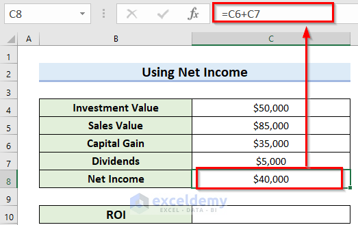 523×329 calculate roi percentage excel methods from www.exceldemy.com
  1150×970 calculate roi excel multiple years from lovelyristin.com
  766×305 calculate roi percentage excel easy ways from www.exceldemy.com
  737×529 calculate roi excel haiper from haipernews.com
  944×708 excel tutorial calculate roi excel excel dashboardscom from dashboardsexcel.com
  477×232 unlocking investment potential calculate roi excel earn from earnandexcel.com
  1024×507 roi template excel exsheets from exsheets.com
  1202×658 roi calculation spreadsheet roi calculation from db-excel.com
  1024×800 roi calculation spreadsheet db excelcom from db-excel.com
  491×471 calculate stock roi manjotattilio from manjotattilio.blogspot.com
  1164×662 roi excel template printable templates from templates.tupuy.com
  1038×696 excel roi template from templates.rjuuc.edu.np
  1024×363 calculate roi manually from www.projectcubicle.com
  1280×720 surprisingly simple steps calculate roi from barnraisersllc.com
  2400×1200 roi formula excel mondaycom blog from monday.com
  768×388 automation roi calculator excel industrial engineering from knowindustrialengineering.com
 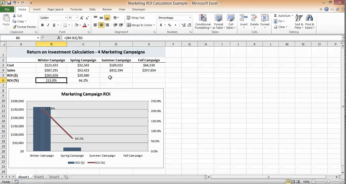 1366×726 roi calculation spreadsheet maxresdefault spreadsheet from db-excel.com
  1280×682 roi template excel from old.sermitsiaq.ag
 How To Calculate ROI For Multiple Investments In Excel was posted in October 14, 2025 at 9:02 pm. If you wanna have it as yours, please click the Pictures and you will go to click right mouse then Save Image As and Click Save and download the How To Calculate ROI For Multiple Investments In Excel Picture.. Don’t forget to share this picture with others via Facebook, Twitter, Pinterest or other social medias! we do hope you'll get inspired by ExcelKayra... Thanks again! If you have any DMCA issues on this post, please contact us!