How To Calculate Weighted Average In Excel Step By Step
How To Calculate Weighted Average In Excel Step By Step - There are a lot of affordable templates out there, but it can be easy to feel like a lot of the best cost a amount of money, require best special design template. Making the best template format choice is way to your template success. And if at this time you are looking for information and ideas regarding the How To Calculate Weighted Average In Excel Step By Step then, you are in the perfect place. Get this How To Calculate Weighted Average In Excel Step By Step for free here. We hope this post How To Calculate Weighted Average In Excel Step By Step inspired you and help you what you are looking for.
Calculating a weighted average in Excel is a common task in various fields like finance, statistics, and academics. It allows you to give more importance (weight) to certain values within a dataset. This guide provides a step-by-step explanation of how to calculate weighted averages in Excel, covering different scenarios and methods.
Understanding Weighted Average
Before diving into the Excel implementation, it’s crucial to understand what a weighted average is. Unlike a simple average (where all values are treated equally), a weighted average considers the relative importance, or “weight,” of each value. This means that some values contribute more to the overall average than others. The formula for a weighted average is:
Weighted Average = (Value1 * Weight1 + Value2 * Weight2 + … + Valuen * Weightn) / (Weight1 + Weight2 + … + Weightn)
In simpler terms, you multiply each value by its corresponding weight, sum these products, and then divide by the sum of all the weights.
Scenario 1: Calculating Weighted Average with Listed Values and Weights
This is the most basic scenario. Imagine you have a list of grades and their respective credit hours (weights).
Step 1: Set up your data in Excel.
Create two columns: one for the values (e.g., Grades) and another for the weights (e.g., Credit Hours). For example:
| Grade | Credit Hours |
|---|---|
| 90 | 3 |
| 85 | 4 |
| 95 | 3 |
| 78 | 2 |
Let’s assume these values are in cells A2:A5 (Grades) and B2:B5 (Credit Hours).
Step 2: Calculate the Weighted Sum (Numerator).
You need to multiply each grade by its corresponding credit hour and sum the results. Excel’s `SUMPRODUCT` function is perfect for this. In an empty cell (e.g., C2), enter the following formula:
=SUMPRODUCT(A2:A5, B2:B5)
This formula does the following:
- `SUMPRODUCT(A2:A5, B2:B5)`: Multiplies the corresponding elements in the two arrays (A2:A5 and B2:B5) and sums the products. In this case: (90*3) + (85*4) + (95*3) + (78*2) = 270 + 340 + 285 + 156 = 1051
Cell C2 will now display the weighted sum (1051).
Step 3: Calculate the Sum of Weights (Denominator).
You need to calculate the total credit hours. Use the `SUM` function in another empty cell (e.g., D2):
=SUM(B2:B5)
This formula sums the values in the range B2:B5. In this case: 3 + 4 + 3 + 2 = 12
Cell D2 will now display the sum of weights (12).
Step 4: Calculate the Weighted Average.
Finally, divide the weighted sum (numerator) by the sum of the weights (denominator). In an empty cell (e.g., E2), enter the following formula:
=C2/D2
This formula divides the value in cell C2 (1051) by the value in cell D2 (12). The result is 87.583333…
Cell E2 will now display the weighted average (approximately 87.58).
Scenario 2: Calculating Weighted Average Directly (Single Formula)
You can combine all the above steps into a single formula for a more concise solution. Instead of using intermediate cells (C2 and D2), you can calculate the weighted average directly.
Step 1: Use the `SUMPRODUCT` and `SUM` functions together.
In an empty cell (e.g., E2), enter the following formula:
=SUMPRODUCT(A2:A5, B2:B5) / SUM(B2:B5)
This formula performs the same calculations as before, but in a single step. It divides the weighted sum (calculated by `SUMPRODUCT`) by the sum of the weights (calculated by `SUM`).
Cell E2 will now display the weighted average (approximately 87.58).
Scenario 3: Handling Missing Weights or Values
Sometimes, your data might have missing weights or values. It’s crucial to handle these cases appropriately to avoid errors or inaccurate results.
Option 1: Treat Missing Weights as Zero
If a weight is missing, you can treat it as zero. This means the corresponding value will not contribute to the weighted average. You can achieve this by manually replacing missing weight values with zero in the weights column.
Option 2: Exclude Rows with Missing Values or Weights
If either the value or the weight is missing, you might want to exclude the entire row from the calculation. You can achieve this using the `IF` function within the `SUMPRODUCT` function, although this can become complex.
To filter the data:
- Select your data range (A1:B5 in our example, including headers).
- Go to the “Data” tab in the Excel ribbon.
- Click on “Filter”.
- Click the dropdown arrow in either the “Grade” or “Credit Hours” column.
- Uncheck the “(Blanks)” option. This will hide any rows where the Grade or Credit Hours cell is empty.
After filtering, the `SUMPRODUCT` and `SUM` formulas will only consider the visible rows, effectively excluding rows with missing values.
Scenario 4: Using a Dynamic Weighting System
Sometimes, weights are not fixed but depend on other factors or conditions. You can use Excel formulas to calculate the weights dynamically.
Example: Weighting based on Volume
Suppose you are calculating the weighted average price of a product, and the weight is determined by the volume of sales. If you have columns for “Price” and “Volume,” you can calculate the weights based on the total volume.
- **Calculate the Weight for Each Row:** In a new column (e.g., Column C), calculate the weight for each row by dividing the volume of that row by the total volume. If your volume data is in B2:B5 and your total volume is in cell B6, the formula in C2 would be: `=B2/$B$6`. Copy this formula down to C3:C5. The `$` signs make B6 an absolute reference, so it doesn’t change when you copy the formula.
- **Calculate the Weighted Average:** Use the `SUMPRODUCT` and `SUM` functions as before, using the Price column (A2:A5) and the calculated weights (C2:C5): `=SUMPRODUCT(A2:A5, C2:C5) / SUM(C2:C5)`
Formatting the Result
The weighted average might have several decimal places. You can format the cell containing the weighted average to display the desired number of decimal places:
- Select the cell containing the weighted average.
- Go to the “Home” tab in the Excel ribbon.
- In the “Number” group, click the “Decrease Decimal” or “Increase Decimal” button to adjust the number of decimal places. Alternatively, click the dropdown and choose “Number” to get more formatting options.
Troubleshooting Common Issues
- **`#DIV/0!` Error:** This error occurs if the sum of the weights is zero. Check your weight values and ensure that at least one weight is greater than zero.
- **Incorrect Result:** Double-check your data and formulas. Make sure you are using the correct ranges in the `SUMPRODUCT` and `SUM` functions, and that the weights are appropriate for your data.
- **Circular Reference:** If you are calculating weights based on other values in the same sheet, be careful to avoid circular references (where a formula depends on its own result).
Conclusion
Calculating weighted averages in Excel is a straightforward process using the `SUMPRODUCT` and `SUM` functions. By following these step-by-step instructions and considering different scenarios, you can accurately calculate weighted averages for various applications.
 556×347 calculate weighted average excel encyclopedia excel from www.encyclopedia-excel.com
 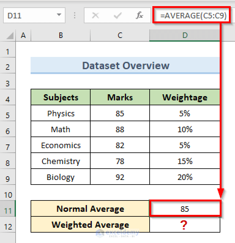 768×794 calculate weighted average excel easy methods from www.exceldemy.com
  590×252 calculate weighted average excel from fundsnetservices.com
  768×440 calculate weighted average excel excel site from thatexcelsite.com
 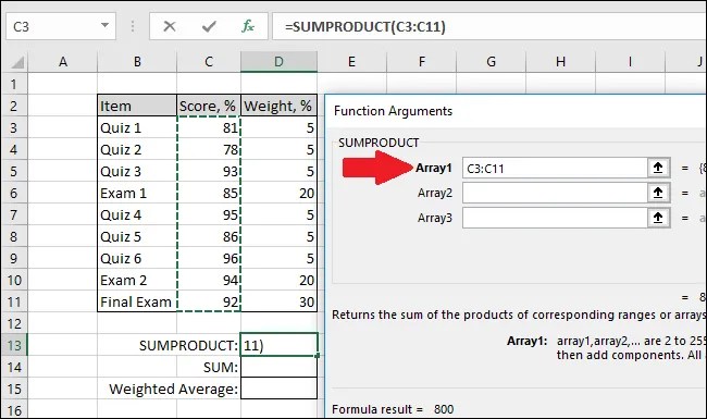 650×385 calculate weighted average excel from www.howtogeek.com
  700×400 weighted average excel formula exceljet from exceljet.net
 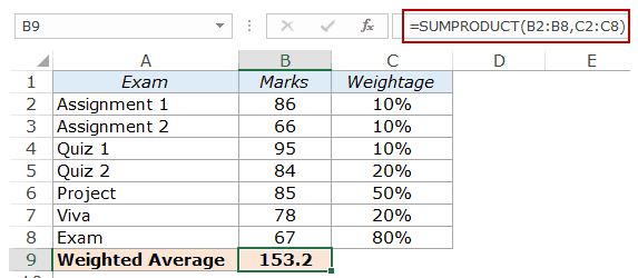 573×250 calculating weighted average excel formulas from trumpexcel.com
  675×282 calculate weighted average excel formula printable from tupuy.com
  239×242 calculate weighted average excel sum sumproduct formulas from www.ablebits.com
  479×230 weighted average excel formula calculate from www.excelmojo.com
  1100×619 calculate weighted average excel howtoexcelnet from howtoexcel.net
  1024×576 calculate weighted average excel easyclick from www.easyclickacademy.com
  1280×720 weighted average excel from fity.club
  1500×619 weighted average formula excel from blog.hubspot.com
  1024×1024 calculate weighted average excel manycoders from manycoders.com
  660×249 calculate weighted average excel geeksforgeeks from adrienj.tinosmarble.com
  600×315 weighted average excel step step tutorial from www.excel-easy.com
  648×449 excel formulas calculate weighted average easy guide hot sex from www.hotzxgirl.com
  534×340 weighted average excel calculate weighted average excel from www.educba.com
 How To Calculate Weighted Average In Excel Step By Step was posted in October 18, 2025 at 4:20 am. If you wanna have it as yours, please click the Pictures and you will go to click right mouse then Save Image As and Click Save and download the How To Calculate Weighted Average In Excel Step By Step Picture.. Don’t forget to share this picture with others via Facebook, Twitter, Pinterest or other social medias! we do hope you'll get inspired by ExcelKayra... Thanks again! If you have any DMCA issues on this post, please contact us!