Home » Excel Templates » How To Combine Match And Index Functions For Complex Lookups In Excel

How To Combine Match And Index Functions For Complex Lookups In Excel

Sunday, February 8th 2026. | Excel Templates

How To Combine Match And Index Functions For Complex Lookups In Excel - There are a lot of affordable templates out there, but it can be easy to feel like a lot of the best cost a amount of money, require best special design template. Making the best template format choice is way to your template success. And if at this time you are looking for information and ideas regarding the How To Combine Match And Index Functions For Complex Lookups In Excel then, you are in the perfect place. Get this How To Combine Match And Index Functions For Complex Lookups In Excel for free here. We hope this post How To Combine Match And Index Functions For Complex Lookups In Excel inspired you and help you what you are looking for.

index match functions excel analytics tuts

Combining MATCH and INDEX for Complex Lookups in Excel

Excel’s lookup functions are powerful tools for retrieving data based on certain criteria. While functions like VLOOKUP and HLOOKUP are widely used, they have limitations, particularly when dealing with dynamic lookup columns or rows. The combination of the MATCH and INDEX functions provides a more flexible and robust alternative, enabling complex lookups that can handle various scenarios with ease.

Understanding MATCH and INDEX Individually

Before diving into their combined use, let’s briefly understand each function individually:

MATCH Function

The MATCH function searches for a specified value within a range and returns the relative position of that value within the range. It doesn’t return the value itself; it returns the index or the position of the matched item.

Syntax: MATCH(lookup_value, lookup_array, [match_type])

lookup_value: The value you want to find.
lookup_array: The range of cells to search within.
[match_type]: (Optional) Specifies how MATCH should find the lookup_value.
- 0 (default): Finds the first value that is exactly equal to lookup_value.
- 1: Finds the largest value that is less than or equal to lookup_value (lookup_array must be sorted in ascending order).
- -1: Finds the smallest value that is greater than or equal to lookup_value (lookup_array must be sorted in descending order).

Example: =MATCH("Apple", A1:A5, 0). If “Apple” is in cell A3, this formula would return 3.

INDEX Function

The INDEX function returns the value of a cell within a range, based on its row and column number. Think of it as a way to pinpoint a specific cell’s content within a larger data set.

Syntax (Array Form): INDEX(array, row_num, [column_num])

array: The range of cells to search within.
row_num: The row number within the array from which to return a value.
[column_num]: (Optional) The column number within the array from which to return a value. If omitted and the array is a single column, column_num is assumed to be 1.

Example: =INDEX(B1:C10, 5, 2) would return the value in the cell at the 5th row and 2nd column of the range B1:C10 (which is cell C5).

Combining MATCH and INDEX: The Power of Dynamic Lookups

The true power emerges when you combine MATCH and INDEX. Instead of manually providing the row or column number in the INDEX function, you use MATCH to dynamically determine these numbers based on your lookup criteria.

General Formula: =INDEX(return_array, MATCH(lookup_value, lookup_array, 0), MATCH(column_header, header_array, 0))

Let’s break down the components:

return_array: The entire data table, excluding headers. This is the range from which you want to retrieve the value.
MATCH(lookup_value, lookup_array, 0): This determines the row number. lookup_value is the value you are searching for in the row lookup. lookup_array is the column where that value should be found.
MATCH(column_header, header_array, 0): This determines the column number. column_header is the header of the column containing the value you want to retrieve. header_array is the row containing the column headers.

Examples of Complex Lookups

1. Two-Way Lookup (Row and Column Criteria)

Imagine a table of sales data with regions as rows and product categories as columns. You want to find the sales figure for a specific region and product category.

Data Table:

	Electronics	Clothing	Home Goods
North	100	50	75
South	120	60	80
East	110	55	70
West	130	65	85

Let’s say the data is in the range A1:D5, with regions in A2:A5 and categories in B1:D1. You want to find the sales for “South” in “Clothing”.

Formula: =INDEX(B2:D5, MATCH("South", A2:A5, 0), MATCH("Clothing", B1:D1, 0))

Explanation:

B2:D5 is the return_array (the sales data).
MATCH("South", A2:A5, 0) finds the row number where “South” is located (row 2).
MATCH("Clothing", B1:D1, 0) finds the column number where “Clothing” is located (column 2).
INDEX(B2:D5, 2, 2) then returns the value in the 2nd row and 2nd column of B2:D5, which is 60.

2. Dynamic Column Lookup

Suppose you have a table of employee data with various columns like “Employee ID,” “Name,” “Department,” and “Salary.” You want to retrieve different information based on a user-selected column name.

Data Table (Example):

Employee ID	Name	Department	Salary
101	Alice Smith	Marketing	60000
102	Bob Johnson	Sales	70000
103	Charlie Brown	IT	80000

Data is in the range A1:D4, headers in A1:D1, and employee IDs in A2:A4. Let’s say the desired column is specified in cell F1 (e.g., “Salary”), and the employee ID to look up is in cell E1 (e.g., 102).

Formula: =INDEX(A2:D4, MATCH(E1, A2:A4, 0), MATCH(F1, A1:D1, 0))

Explanation:

A2:D4 is the return_array (employee data).
MATCH(E1, A2:A4, 0) finds the row number where the employee ID in E1 (102) is found (row 2).
MATCH(F1, A1:D1, 0) finds the column number corresponding to the column name in F1 (“Salary”) (column 4).
INDEX(A2:D4, 2, 4) returns the value in the 2nd row and 4th column of A2:D4, which is 70000.

If you change the value in F1 to “Department,” the formula will automatically return “Sales.”

3. Handling Errors with IFERROR

When the MATCH function can’t find the lookup_value, it returns an error (#N/A). To handle these errors gracefully, you can wrap the entire INDEX/MATCH formula within an IFERROR function.

Example: Using the employee data example above:

=IFERROR(INDEX(A2:D4, MATCH(E1, A2:A4, 0), MATCH(F1, A1:D1, 0)), "Not Found")

If either MATCH function returns an error, the formula will display “Not Found” instead of #N/A.

Advantages of INDEX and MATCH over VLOOKUP/HLOOKUP

Flexibility: INDEX/MATCH isn’t restricted to looking up values in the leftmost column (as with VLOOKUP) or the topmost row (as with HLOOKUP). You can search in any column or row.
Column Insertion/Deletion: INDEX/MATCH is less prone to breaking when columns are inserted or deleted in your data table. VLOOKUP relies on a fixed column index, which can be easily disrupted by changes to the table structure. INDEX/MATCH uses the header row to find the correct column, making it more resilient.
Performance: In some cases, INDEX/MATCH can be more efficient than VLOOKUP, especially with large datasets, as it directly accesses the required data rather than iterating through the table.

Conclusion

The combination of MATCH and INDEX provides a powerful and flexible alternative to VLOOKUP and HLOOKUP in Excel. By dynamically determining row and column numbers, this approach allows for more complex and robust lookups that are less susceptible to errors and more adaptable to changes in your data structure. Understanding and mastering this technique will significantly enhance your data analysis capabilities in Excel.

1337×443 index match functions excel analytics tuts from www.analytics-tuts.com

651×463 combine index match functions excel from tipsmake.com

640×443 index match excel function combination sheetgo blog from blog.sheetgo.com

1956×491 multi condition lookups ways excel from professor-excel.com

1350×1220 combining index match excel maven from www.excelmaven.com

1375×943 vlookups match indexmatch xlookup from intellectualrabbithole.com

624×395 lookup formula excel index match teachexcelcom from www.teachexcel.com

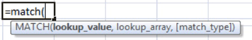500×81 complete guide index match flexible lookups excel from www.xelplus.com

How To Combine Match And Index Functions For Complex Lookups In Excel was posted in February 8, 2026 at 1:32 am. If you wanna have it as yours, please click the Pictures and you will go to click right mouse then Save Image As and Click Save and download the How To Combine Match And Index Functions For Complex Lookups In Excel Picture.. Don’t forget to share this picture with others via Facebook, Twitter, Pinterest or other social medias! we do hope you'll get inspired by ExcelKayra... Thanks again! If you have any DMCA issues on this post, please contact us!