How To Create A Balance Sheet In Excel For Beginners
How To Create A Balance Sheet In Excel For Beginners - There are a lot of affordable templates out there, but it can be easy to feel like a lot of the best cost a amount of money, require best special design template. Making the best template format choice is way to your template success. And if at this time you are looking for information and ideas regarding the How To Create A Balance Sheet In Excel For Beginners then, you are in the perfect place. Get this How To Create A Balance Sheet In Excel For Beginners for free here. We hope this post How To Create A Balance Sheet In Excel For Beginners inspired you and help you what you are looking for.
Here’s an HTML formatted guide on creating a balance sheet in Excel, geared towards beginners:
Creating a Balance Sheet in Excel for Beginners
The balance sheet is a snapshot of a company’s assets, liabilities, and equity at a specific point in time. It follows the basic accounting equation: Assets = Liabilities + Equity. Creating a balance sheet in Excel can seem daunting, but with a little guidance, it becomes a manageable task. This tutorial will walk you through the process step-by-step.
1. Understanding the Balance Sheet Structure
Before jumping into Excel, it’s crucial to understand the different components of a balance sheet:
- Assets: What the company owns. Divided into:
- Current Assets: Assets that can be converted to cash within a year (e.g., cash, accounts receivable, inventory).
- Non-Current Assets (Fixed Assets): Assets with a lifespan of more than a year (e.g., property, plant, and equipment).
- Liabilities: What the company owes to others. Divided into:
- Current Liabilities: Debts due within a year (e.g., accounts payable, salaries payable, short-term loans).
- Non-Current Liabilities (Long-Term Liabilities): Debts due beyond a year (e.g., long-term loans, bonds payable).
- Equity: The owners’ stake in the company (also known as shareholders’ equity or owner’s equity). Includes:
- Common Stock: Value of shares issued to owners.
- Retained Earnings: Accumulated profits kept by the company.
2. Setting Up Your Excel Worksheet
- Open Excel and Create a New Worksheet: Start with a blank sheet.
- Title Your Balance Sheet: In cell A1, type the company name (e.g., “Acme Corp”) and in A2, type “Balance Sheet” followed by the date (e.g., “As of December 31, 2023”).
- Label Columns: In row 4, start labeling columns. A common setup is:
- Column A: Account Name (e.g., “Cash,” “Accounts Receivable”)
- Column B: Amount (e.g., “$10,000,” “$5,000”)
3. Entering Asset Data
- Start with Current Assets: In column A, starting from row 6, list your current assets:
- Cash
- Accounts Receivable
- Inventory
- Prepaid Expenses
- Enter Corresponding Amounts: In column B, enter the dollar amount for each asset. For example:
- B6:
=10000(for Cash) - B7:
=5000(for Accounts Receivable) - B8:
=12000(for Inventory) - B9:
=2000(for Prepaid Expenses)
- B6:
- Calculate Total Current Assets: Below the last current asset, label a cell (e.g., A10) as “Total Current Assets.” In the corresponding cell in column B (B10), use the
SUMfunction to add up all current assets. For example:=SUM(B6:B9). - List Non-Current Assets (Fixed Assets): Below the total current assets, list your non-current assets, also known as fixed assets:
- Property, Plant & Equipment (PP&E)
- Less: Accumulated Depreciation
- Net PP&E
- Land
- Buildings
- Equipment
- Enter Corresponding Amounts: In column B, enter the dollar amount for each non-current asset. For example:
- B12:
=50000(for Property, Plant & Equipment (PP&E)) - B13:
=10000(for Less: Accumulated Depreciation)
- B12:
- Calculate Net PP&E: Net PP&E equals PP&E minus accumulated depreciation. If PP&E is in B12, and Accumulated Depreciation is in B13, enter the following formula in B14:
=B12-B13. - Calculate Total Non-Current Assets: Below the last fixed asset, label a cell (e.g., A17) as “Total Fixed Assets.” In the corresponding cell in column B (B17), use the
SUMfunction to add up all fixed assets. For example:=SUM(B14:B16)(assuming land, buildings, and equipment). If you only have Net PP&E, the formula would just be=B14. - Calculate Total Assets: Label a cell (e.g., A18) as “Total Assets.” In the corresponding cell in column B (B18), add the total current assets and total fixed assets. For example:
=B10+B17.
4. Entering Liability Data
- Start with Current Liabilities: Below the total assets section, list your current liabilities:
- Accounts Payable
- Salaries Payable
- Short-Term Loans
- Enter Corresponding Amounts: In column B, enter the amounts for each liability. For example:
- B20:
=8000(for Accounts Payable) - B21:
=3000(for Salaries Payable) - B22:
=4000(for Short-Term Loans)
- B20:
- Calculate Total Current Liabilities: Label a cell (e.g., A23) as “Total Current Liabilities.” In the corresponding cell in column B (B23), use the
SUMfunction:=SUM(B20:B22). - List Non-Current Liabilities (Long-Term Liabilities): Below the total current liabilities, list your long-term liabilities:
- Long-Term Loans
- Bonds Payable
- Enter Corresponding Amounts: In column B, enter the amounts for each long-term liability. For example:
- B25:
=20000(for Long-Term Loans) - B26:
=15000(for Bonds Payable)
- B25:
- Calculate Total Long-Term Liabilities: Label a cell (e.g., A27) as “Total Long-Term Liabilities.” In the corresponding cell in column B (B27), use the
SUMfunction:=SUM(B25:B26). If you only have one long-term liability, the formula would be simply=B25(or whatever the appropriate cell is). - Calculate Total Liabilities: Label a cell (e.g., A28) as “Total Liabilities.” In the corresponding cell in column B (B28), add the total current liabilities and total long-term liabilities:
=B23+B27.
5. Entering Equity Data
- List Equity Accounts: Below the total liabilities, list your equity accounts:
- Common Stock
- Retained Earnings
- Enter Corresponding Amounts: In column B, enter the amounts for each equity account. For example:
- B30:
=25000(for Common Stock) - B31:
=30000(for Retained Earnings)
- B30:
- Calculate Total Equity: Label a cell (e.g., A32) as “Total Equity.” In the corresponding cell in column B (B32), add the values of common stock and retained earnings:
=B30+B31.
6. Verifying the Balance Sheet Equation
- Calculate Total Liabilities and Equity: Label a cell (e.g., A34) as “Total Liabilities & Equity”. In the corresponding cell in column B (B34), add the total liabilities and total equity:
=B28+B32. - Compare with Total Assets: Verify that the value in cell B34 (Total Liabilities & Equity) is equal to the value in cell B18 (Total Assets). If they are not equal, you have an error somewhere in your data entry or calculations.
7. Formatting and Final Touches
- Format Numbers: Select the cells containing dollar amounts and format them as currency (e.g., using the dollar sign and two decimal places). Use the “Accounting” number format for a professional look.
- Add Borders and Shading: Use borders to separate sections and shading to highlight totals for better readability.
- Adjust Column Widths: Adjust the column widths so that all labels and values are fully visible.
By following these steps, you can create a basic balance sheet in Excel. Remember to double-check your data entry and calculations to ensure accuracy. As you become more comfortable, you can explore more advanced features and formulas in Excel to create more sophisticated financial statements.
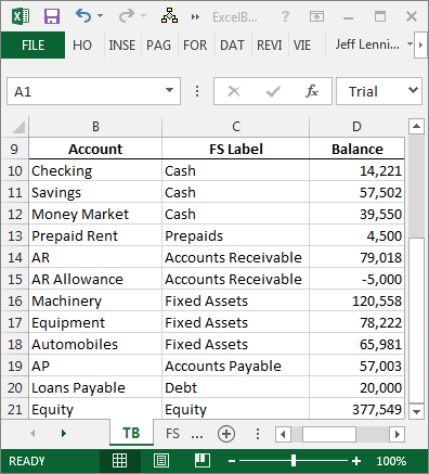 396×437 create balance sheet excel excel university from www.excel-university.com
  620×1000 create balance sheet guide excel capital from www.excelcapmanagement.com
  1024×1024 balance sheet format excel formulas khairilmazri balance from db-excel.com
  1280×720 balance sheet template excel db excelcom from db-excel.com
  876×723 simple balance sheet spreadsheet excel fppt from www.free-power-point-templates.com
  580×420 simple balance sheet template excel from www.free-power-point-templates.com
 How To Create A Balance Sheet In Excel For Beginners was posted in December 4, 2025 at 7:31 pm. If you wanna have it as yours, please click the Pictures and you will go to click right mouse then Save Image As and Click Save and download the How To Create A Balance Sheet In Excel For Beginners Picture.. Don’t forget to share this picture with others via Facebook, Twitter, Pinterest or other social medias! we do hope you'll get inspired by ExcelKayra... Thanks again! If you have any DMCA issues on this post, please contact us!