How To Create A Dynamic Heat Map In Excel
How To Create A Dynamic Heat Map In Excel - There are a lot of affordable templates out there, but it can be easy to feel like a lot of the best cost a amount of money, require best special design template. Making the best template format choice is way to your template success. And if at this time you are looking for information and ideas regarding the How To Create A Dynamic Heat Map In Excel then, you are in the perfect place. Get this How To Create A Dynamic Heat Map In Excel for free here. We hope this post How To Create A Dynamic Heat Map In Excel inspired you and help you what you are looking for.
“`html
Creating a Dynamic Heat Map in Excel
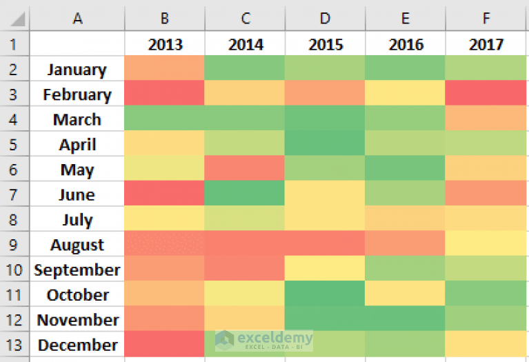
Heat maps are powerful visual tools that use color gradients to represent data density or magnitude. In Excel, you can create dynamic heat maps that automatically update as your underlying data changes. This guide will walk you through the process, leveraging Excel’s conditional formatting features to achieve a visually compelling and interactive heat map.
1. Preparing Your Data
The first step is ensuring your data is structured appropriately for a heat map. Typically, heat maps are used to represent data in a two-dimensional grid. Your data should ideally be organized with rows representing one category and columns representing another. The cells within the grid will contain the values you want to visualize with the heat map’s color gradient.
Example: Imagine you have sales data for different products across various regions. Your rows could represent products (e.g., “Product A”, “Product B”, “Product C”) and your columns could represent regions (e.g., “North”, “South”, “East”, “West”). Each cell would contain the sales figure for a particular product in a specific region.
Make sure your data is clean and consistent. Remove any blank rows or columns that might interfere with the formatting. Standardize data formats (e.g., ensure all numbers are formatted as numbers, all dates are formatted as dates).
2. Selecting Your Data Range
Once your data is ready, select the range of cells that you want to apply the heat map to. This is the rectangular area that will be colored based on the data values within it. Don’t include row or column headers in your selection; just select the data itself.
3. Applying Conditional Formatting
Excel’s conditional formatting feature is the key to creating a dynamic heat map. Here’s how to access it:
- Go to the “Home” tab on the Excel ribbon.
- In the “Styles” group, click on “Conditional Formatting.”
- A dropdown menu will appear. Choose “Color Scales.”
Excel offers several pre-defined color scales. These scales generally use a range of colors, often from green (low values) to red (high values), or blue (low values) to red (high values). You can choose a pre-defined scale that suits your needs, or you can create a custom color scale for greater control.
4. Choosing a Pre-Defined Color Scale
For a quick and easy heat map, selecting a pre-defined color scale is a good starting point. Hover your mouse over the different color scale options in the dropdown menu. Excel will provide a live preview of how the heat map will look on your selected data range. Choose a scale that effectively highlights the differences in your data values.
Commonly used pre-defined scales include:
- Green-Yellow-Red Color Scale: This scale is intuitive, with green representing low values, yellow representing mid-range values, and red representing high values.
- Red-Yellow-Green Color Scale: This is the reverse of the previous scale.
- Blue-White-Red Color Scale: This scale can be effective for highlighting both positive and negative values, with white representing values close to zero.
After selecting a color scale, Excel will automatically apply the formatting to your data. The color of each cell will now correspond to its value, creating the heat map effect.
5. Customizing Your Color Scale (Advanced)
For more granular control over your heat map, you can customize the color scale. To do this, after selecting “Conditional Formatting” and “Color Scales,” choose “More Rules…” at the bottom of the dropdown menu. This will open the “New Formatting Rule” dialog box.
- Under “Select a Rule Type,” ensure “Format all cells based on their values” is selected.
- Under “Format Style,” choose “3-Color Scale” (or “2-Color Scale” if you prefer a simpler gradient).
- Now you can customize the “Minimum,” “Midpoint,” and “Maximum” values, along with their corresponding colors.
Value Types:
- Lowest Value/Highest Value: These options automatically use the lowest and highest values in your selected data range.
- Number: You can specify a specific numerical value for the minimum, midpoint, or maximum.
- Percent: You can use a percentage relative to the range of values in your data. For example, “Percent 25” would represent the value at the 25th percentile.
- Percentile: Similar to percent, but calculates the percentile based on the data distribution.
- Formula: You can use an Excel formula to dynamically calculate the minimum, midpoint, or maximum values. This is particularly useful for creating highly dynamic heat maps that respond to changes in other parts of your spreadsheet.
Colors:
Click on the color swatches next to each value (Minimum, Midpoint, Maximum) to choose the colors you want to use for your heat map. Select colors that are visually distinct and that clearly represent the range of values you are visualizing. Consider using colorblind-friendly palettes.
Midpoint: The midpoint allows you to define a neutral value in your heat map. Values above the midpoint will be colored according to the gradient between the midpoint color and the maximum color, while values below the midpoint will be colored according to the gradient between the midpoint color and the minimum color.
6. Managing and Editing Existing Heat Maps
To edit an existing heat map, follow these steps:
- Select the data range that has the heat map applied.
- Go to “Home” -> “Conditional Formatting” -> “Manage Rules…”
- In the “Conditional Formatting Rules Manager” dialog box, make sure “This Worksheet” is selected in the “Show formatting rules for:” dropdown.
- You will see a list of the conditional formatting rules applied to your selected range. Select the heat map rule you want to edit and click “Edit Rule…”
- This will bring you back to the “Edit Formatting Rule” dialog box, where you can modify the color scale, value types, and colors as described in step 5.
You can also delete a heat map rule from the “Conditional Formatting Rules Manager” by selecting the rule and clicking “Delete Rule.”
7. Tips for Effective Heat Maps
- Choose appropriate color scales: Consider the nature of your data and the message you want to convey when selecting colors.
- Use consistent data formatting: Ensure all numbers are formatted consistently to avoid misinterpretations.
- Avoid overly complex color scales: Too many colors can make the heat map difficult to interpret. Stick to a simple and clear gradient.
- Consider your audience: Choose colors and a layout that will be easily understood by your target audience.
- Label your axes clearly: Make sure the rows and columns are clearly labeled so that viewers can understand the context of the data.
- Use data labels sparingly: Adding data labels to every cell can clutter the heat map. Consider adding labels only to cells with the highest or lowest values, or to cells that are particularly important.
By following these steps, you can create dynamic and informative heat maps in Excel that will help you visualize your data and gain valuable insights.
“`
 767×525 create heat map excel methods exceldemy from www.exceldemy.com
  489×417 heat map excel step step tutorial from www.excel-easy.com
  438×800 building dynamic heat map excel softarchive from sanet.st
 How To Create A Dynamic Heat Map In Excel was posted in July 31, 2025 at 12:04 am. If you wanna have it as yours, please click the Pictures and you will go to click right mouse then Save Image As and Click Save and download the How To Create A Dynamic Heat Map In Excel Picture.. Don’t forget to share this picture with others via Facebook, Twitter, Pinterest or other social medias! we do hope you'll get inspired by ExcelKayra... Thanks again! If you have any DMCA issues on this post, please contact us!