How To Create A Gantt Chart In Excel For Project Management
How To Create A Gantt Chart In Excel For Project Management - There are a lot of affordable templates out there, but it can be easy to feel like a lot of the best cost a amount of money, require best special design template. Making the best template format choice is way to your template success. And if at this time you are looking for information and ideas regarding the How To Create A Gantt Chart In Excel For Project Management then, you are in the perfect place. Get this How To Create A Gantt Chart In Excel For Project Management for free here. We hope this post How To Create A Gantt Chart In Excel For Project Management inspired you and help you what you are looking for.
“`html
Creating a Gantt Chart in Excel for Project Management
Gantt charts are powerful visual tools for project management, offering a clear overview of project timelines, tasks, dependencies, and milestones. While dedicated project management software offers advanced features, Microsoft Excel provides a readily accessible and customizable platform for creating basic Gantt charts. This guide details how to construct a functional Gantt chart in Excel to effectively manage your projects.
Understanding the Essentials
Before diving into the steps, it’s crucial to understand the core components of a Gantt chart:
- Tasks: The individual activities that need to be completed to achieve the project goals.
- Start Date: The date when a task is scheduled to begin.
- Duration: The estimated time required to complete a task (usually measured in days or weeks).
- End Date: The date when a task is expected to be finished (calculated based on the start date and duration).
- Dependencies: Relationships between tasks, indicating which tasks need to be completed before others can begin.
- Timeline: A horizontal axis representing the project’s overall duration, showing dates or weeks.
- Bars: Visual representations of tasks, extending along the timeline to indicate their start and end dates.
Step-by-Step Guide to Creating a Gantt Chart in Excel
1. Data Preparation
The foundation of your Gantt chart is a well-structured data table. Open a new Excel worksheet and create the following columns:
- Task Name: List each task clearly and concisely.
- Start Date: Enter the planned start date for each task. Ensure the date format is consistent (e.g., MM/DD/YYYY).
- Duration (Days): Input the estimated number of days required to complete each task.
- End Date (Calculated): This column will automatically calculate the end date using the formula:
=Start Date + Duration - 1. Subtracting 1 ensures that the end date is inclusive of the start date. Apply this formula to all rows in the End Date column.
Optionally, you can add additional columns like “Assigned To,” “Status,” “Dependencies,” or “Notes” for more detailed project tracking.
2. Creating the Basic Chart
Excel’s Stacked Bar Chart will be adapted to simulate a Gantt chart. Follow these steps:
- Select Data: Select the “Task Name” and “Start Date” columns (including headers).
- Insert Chart: Go to the “Insert” tab on the Excel ribbon. In the “Charts” group, click on the “Insert Column or Bar Chart” dropdown menu. Choose “Stacked Bar.”
- Add Duration Data: Right-click on the chart and select “Select Data.”
- In the “Select Data Source” window, click “Add.”
- For “Series name,” type “Duration.”
- For “Series values,” select the cells in the “Duration (Days)” column (excluding the header).
- Click “OK” in both windows.
You’ll now have a Stacked Bar chart where each task has two bars: one representing the start date (colored) and another representing the duration (also colored).
3. Formatting the Chart to Resemble a Gantt Chart
The default chart needs significant formatting to look like a proper Gantt chart:
- Hide the Start Date Bars: Click on one of the “Start Date” bars in the chart. Right-click and select “Format Data Series.”
- In the “Format Data Series” pane, go to the “Fill & Line” tab (the paint bucket icon).
- Under “Fill,” select “No fill.” This will make the Start Date bars invisible, effectively positioning the Duration bars at the correct start dates.
- Optionally, under “Border,” select “No line” for a cleaner look.
- Format the Task Axis: Currently, the task names are on the wrong side and in reverse order.
- Click on the vertical axis (with task names). Right-click and select “Format Axis.”
- In the “Format Axis” pane, under “Axis Options,” check the boxes for “Categories in reverse order” and “Horizontal axis crosses at maximum category.” This will place the task names on the left and in the correct order.
- Adjust the Date Axis: The date axis needs to be adjusted to display the correct range.
- Click on the horizontal axis (with dates). Right-click and select “Format Axis.”
- In the “Format Axis” pane, under “Axis Options,” set the “Minimum” and “Maximum” values. To determine appropriate values:
- For the “Minimum,” enter the numerical value of the project’s overall start date. You can find this by entering the project’s earliest start date into a cell and formatting that cell as “General.” The resulting number is what you’ll use as the minimum.
- For the “Maximum,” calculate the project’s end date by finding the latest end date of all tasks, and similarly format that date cell as “General” to get its numerical value. Use this as the maximum.
- Adjust the “Units” (Major) to a suitable increment, such as 7 for weekly increments or 30 for monthly increments.
- Under “Number,” select a more readable date format.
- Customize Bar Colors: Click on the “Duration” bars. Right-click and select “Format Data Series.” In the “Fill & Line” tab, choose a desired color for the bars. You can customize the color for each task by clicking on individual bars after selecting the series.
4. Adding Dependencies (Optional)
Excel doesn’t natively support dependency lines. However, you can manually add them using shapes:
- Go to the “Insert” tab and click on “Shapes.” Choose a line or arrow shape.
- Draw lines connecting the end of one task’s bar to the start of the dependent task’s bar.
- Adjust the line style, color, and weight as needed.
Keep in mind that these lines are static and won’t automatically update if task dates change. This manual approach works best for simple dependencies.
5. Enhancements and Refinements
- Add a Legend: If you’ve used different colors to represent task types or statuses, add a legend to clarify the color coding.
- Add Milestones: Represent key project milestones by adding a special shape (e.g., a diamond) at the corresponding date on the chart.
- Data Validation: Use data validation to restrict the possible values for certain columns (e.g., ensuring that duration is always a positive number).
- Conditional Formatting: Use conditional formatting to highlight tasks based on their status (e.g., overdue tasks in red).
Conclusion
While Excel’s Gantt chart functionality isn’t as sophisticated as dedicated project management tools, it provides a practical and accessible way to visualize project timelines and manage tasks. By following these steps, you can create a functional Gantt chart in Excel to effectively plan, track, and manage your projects.
“`
 1280×577 project management gantt excel from www.ganttexcel.com
  1022×556 excel gantt chart prioritization blog from appfluence.com
  1577×636 create gantt charts excel easy step step guide from www.ganttexcel.com
  1634×986 project management excel gantt chart template excel templates from www.exceltemplate123.us
 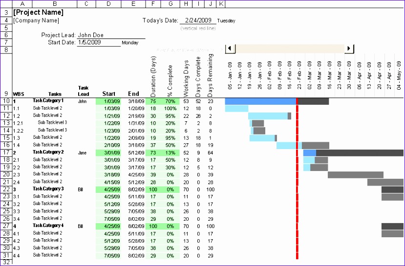 829×546 project management excel gantt chart template excel templates from www.exceltemplate123.us
  1072×804 gantt chart timeline template excel db excelcom from db-excel.com
  1588×814 excel gantt chart template easy project management project etsy from www.etsy.com
 How To Create A Gantt Chart In Excel For Project Management was posted in October 6, 2025 at 9:15 am. If you wanna have it as yours, please click the Pictures and you will go to click right mouse then Save Image As and Click Save and download the How To Create A Gantt Chart In Excel For Project Management Picture.. Don’t forget to share this picture with others via Facebook, Twitter, Pinterest or other social medias! we do hope you'll get inspired by ExcelKayra... Thanks again! If you have any DMCA issues on this post, please contact us!