How To Create A Personal Finance Spreadsheet In Excel
How To Create A Personal Finance Spreadsheet In Excel - There are a lot of affordable templates out there, but it can be easy to feel like a lot of the best cost a amount of money, require best special design template. Making the best template format choice is way to your template success. And if at this time you are looking for information and ideas regarding the How To Create A Personal Finance Spreadsheet In Excel then, you are in the perfect place. Get this How To Create A Personal Finance Spreadsheet In Excel for free here. We hope this post How To Create A Personal Finance Spreadsheet In Excel inspired you and help you what you are looking for.
Creating a Personal Finance Spreadsheet in Excel
Taking control of your finances can feel daunting, but a well-organized personal finance spreadsheet is a powerful tool that can simplify the process. Excel, readily available and familiar to many, offers a flexible platform to track income, expenses, savings, and investments. This guide walks you through creating a comprehensive personal finance spreadsheet from scratch.
Step 1: Setting Up the Basic Structure
Begin by opening a new Excel workbook. Think of each worksheet as a separate “dashboard” for different aspects of your finances. A good starting point includes worksheets for:
- Summary: A high-level overview of your financial situation.
- Income: Tracks all sources of income.
- Expenses: Categorizes and tracks all expenses.
- Savings: Monitors your savings goals and progress.
- Debt: Manages your outstanding debts.
- Investments: Tracks your investment portfolio.
Rename the default “Sheet1,” “Sheet2,” etc., tabs at the bottom of the screen to reflect these categories. This will make navigation much easier.
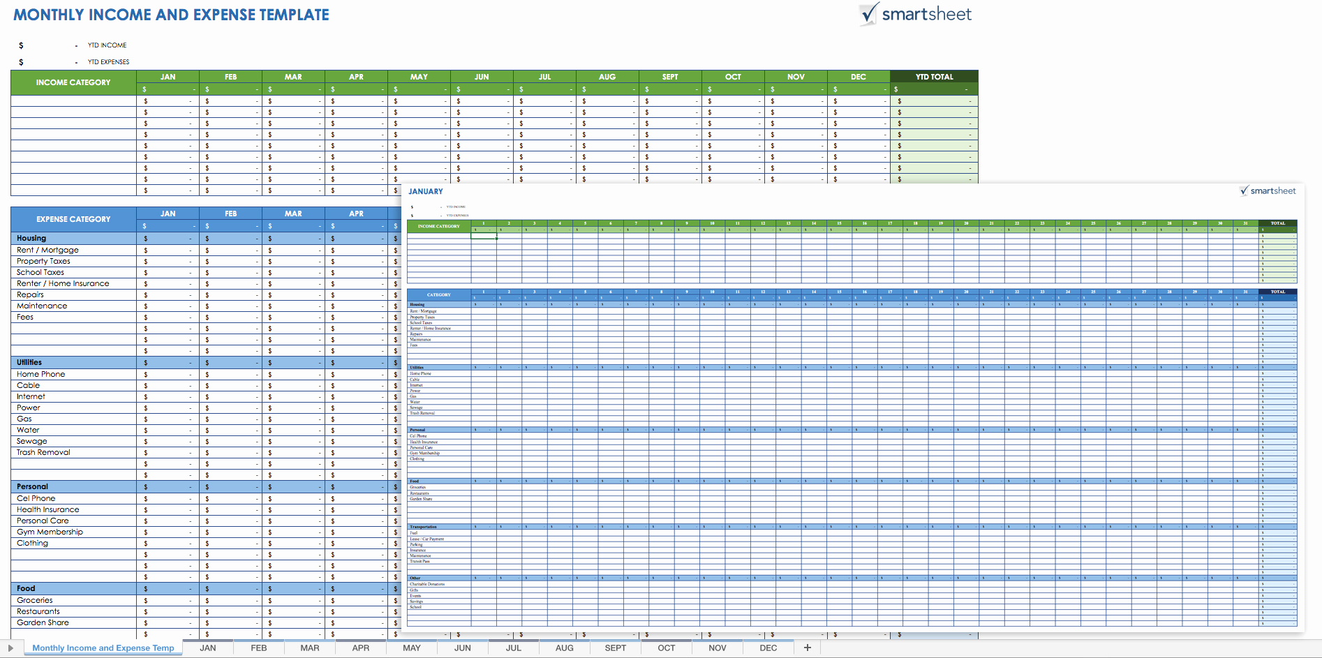
Step 2: Building the Income Worksheet
The Income worksheet should list all sources of your income. Structure it with columns for:
- Date: The date the income was received.
- Source: The origin of the income (e.g., Salary, Freelance, Investment Income).
- Description: A brief explanation (e.g., “Paycheck from Acme Corp,” “Freelance Project – Website Design”).
- Amount: The amount of income received.
Enter your income details for each pay period or income event. At the bottom of the column, use the =SUM() function to calculate your total income for the month or year. For example, if your income amounts are in column D, starting from D2, the formula would be =SUM(D2:D100) (adjust the range as needed).
Consider adding a column for “Planned” versus “Actual” income. This allows you to compare your expected income with what you actually received, helping you identify potential discrepancies.
Step 3: Creating the Expenses Worksheet
This is arguably the most crucial worksheet. It requires detailed categorization of your spending. Start by defining broad categories such as:
- Housing: Rent/Mortgage, Property Taxes, Insurance, Maintenance.
- Transportation: Car Payments, Gas, Insurance, Public Transportation, Maintenance.
- Food: Groceries, Dining Out.
- Utilities: Electricity, Gas, Water, Internet, Phone.
- Healthcare: Insurance Premiums, Doctor Visits, Prescriptions.
- Personal: Clothing, Entertainment, Hobbies, Personal Care.
- Debt Payments: Credit Card Payments, Loan Payments.
- Savings: Contributions to Savings Accounts, Investments.
Within each category, you can create subcategories for more granular tracking. The Expenses worksheet should include columns for:
- Date: The date of the expense.
- Category: The broad expense category.
- Subcategory: The specific expense subcategory.
- Description: A brief explanation (e.g., “Grocery Shopping at Safeway,” “Dinner at Italian Restaurant”).
- Amount: The amount of the expense.
- Payment Method: How you paid (e.g., Credit Card, Debit Card, Cash).
Use the =SUMIF() function to automatically calculate the total spending within each category and subcategory. For example, to calculate the total spent on “Groceries” (assuming categories are in column B and amounts are in column E), you would use the formula =SUMIF(B:B, "Food", E:E). You can then create a summary table at the top of the worksheet showing your total spending per category.
Step 4: Tracking Savings
The Savings worksheet monitors your progress towards your savings goals. Columns to include are:
- Goal: The specific savings goal (e.g., Emergency Fund, Down Payment, Retirement).
- Target Amount: The total amount you need to save.
- Current Amount: The amount you have currently saved.
- Monthly Contribution: The amount you contribute each month.
- Date: The date of the contribution.
- Notes: Any relevant notes (e.g., “High-Yield Savings Account,” “Roth IRA”).
Calculate the “Remaining Amount” by subtracting the “Current Amount” from the “Target Amount.” This helps you visualize how close you are to reaching your goals. Consider adding a column to calculate the estimated time to reach your goal based on your monthly contributions.
Step 5: Managing Debt
The Debt worksheet helps you track and manage your outstanding debts. Key columns include:
- Creditor: The lender (e.g., “Chase Credit Card,” “Bank of America Auto Loan”).
- Type of Debt: (e.g., Credit Card, Auto Loan, Student Loan).
- Original Loan Amount: The initial loan amount.
- Current Balance: The outstanding balance.
- Interest Rate: The annual interest rate.
- Minimum Payment: The minimum monthly payment.
- Payment Due Date: The date the payment is due.
Calculate the total debt by summing the “Current Balance” column. You can also use Excel’s built-in financial functions (e.g., PMT, IPMT, PPMT) to calculate monthly payments, interest paid, and principal paid on each debt. This allows you to develop a debt repayment strategy.
Step 6: Monitoring Investments
The Investments worksheet provides an overview of your investment portfolio. Include columns for:
- Investment Type: (e.g., Stocks, Bonds, Mutual Funds, Real Estate).
- Asset: The specific investment (e.g., “Apple Stock,” “Vanguard S&P 500 ETF”).
- Quantity: The number of shares or units held.
- Purchase Price: The price at which you bought the asset.
- Current Price: The current market price of the asset.
- Market Value: The current total value of the investment (Quantity * Current Price).
- Gain/Loss: The profit or loss on the investment (Market Value – (Quantity * Purchase Price)).
You can use Excel’s “Stocks” data type to automatically retrieve current stock prices and other financial data. This feature allows you to keep your portfolio up-to-date with minimal effort. Calculate your total portfolio value by summing the “Market Value” column.
Step 7: Creating the Summary Worksheet
The Summary worksheet consolidates key information from the other worksheets to provide a high-level overview of your financial health. Include the following:
- Total Income: (Linked from the Income worksheet).
- Total Expenses: (Linked from the Expenses worksheet).
- Net Income: (Total Income – Total Expenses).
- Total Savings: (Linked from the Savings worksheet).
- Total Debt: (Linked from the Debt worksheet).
- Total Investment Value: (Linked from the Investments worksheet).
Use formulas to calculate key financial ratios, such as your savings rate (Total Savings / Total Income) and debt-to-income ratio (Total Debt / Total Income). These ratios provide insights into your financial strengths and weaknesses.
Step 8: Adding Visualizations and Charts
Visualizations can make your spreadsheet more engaging and easier to understand. Use Excel’s charting tools to create charts and graphs that illustrate your financial data. Some useful chart types include:
- Pie Chart: To show the breakdown of your expenses by category.
- Line Chart: To track your income and expenses over time.
- Bar Chart: To compare your savings progress against your goals.
Select the data you want to visualize and then choose the appropriate chart type from the “Insert” tab. Customize the chart’s appearance to make it visually appealing and informative.
Step 9: Automating and Maintaining Your Spreadsheet
To maximize the usefulness of your spreadsheet, automate as much as possible. Use Excel’s features such as data validation, conditional formatting, and formulas to streamline data entry and analysis.
- Data Validation: To create drop-down lists for categories and subcategories in the Expenses worksheet, ensuring consistent data entry.
- Conditional Formatting: To highlight cells that meet certain criteria, such as expenses exceeding a budget or debt balances nearing zero.
- Formulas: To automatically calculate totals, balances, and other key metrics.
Regularly update your spreadsheet with new income, expenses, and investment data. Set aside a specific time each week or month to review your finances and make any necessary adjustments to your budget or financial plan.
Conclusion
Creating and maintaining a personal finance spreadsheet in Excel requires an initial investment of time and effort, but the rewards are significant. By tracking your income, expenses, savings, and investments, you gain a clear understanding of your financial situation, enabling you to make informed decisions and achieve your financial goals.
 1894×943 personal finance spreadsheet excel resourcesaver personal finance from db-excel.com
  1156×868 personal finance spreadsheet db excelcom from db-excel.com
  474×366 personal finance spreadsheet template db excelcom from db-excel.com
  1024×791 personal finance spreadsheet template db excelcom from db-excel.com
  1024×1024 personal finance spreadsheet spreadsheet downloa personal finance from db-excel.com
  1024×618 personal finance spreadsheet excel db excelcom from db-excel.com
  1024×640 personal finance spreadsheet templates excelxocom from excelxo.com
  1024×791 personal finance spreadsheet templates db excelcom from db-excel.com
 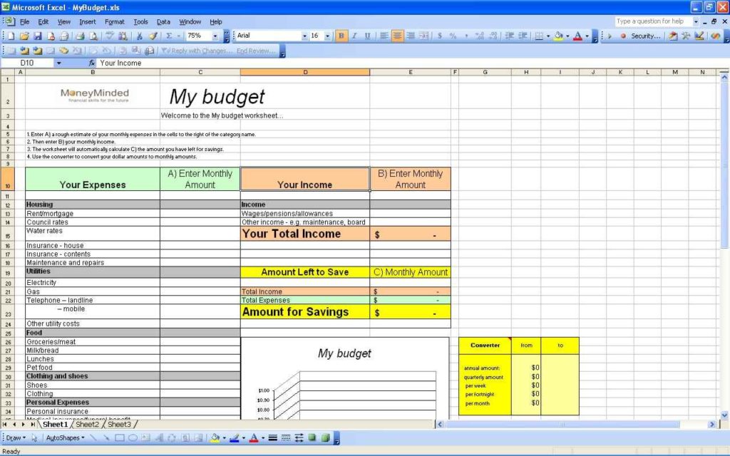 1024×640 personal budget spreadsheet excel db excelcom from db-excel.com
  1692×1692 personal finance spreadsheet spreadsheet downloa personal from db-excel.com
  600×303 personal finance spreadsheet template spreadsheet templates from excelxo.com
  1496×970 personal finance spreadsheet excel financial planning sheet db excelcom from db-excel.com
  1920×1030 personal finance excel spreadsheet template luz templates from www.luztemplates.com
  750×715 personal finance spreadsheet template google sheets from thegoodocs.com
  1080×1080 personal finance excel spreadsheet templates managing money from www.pinterest.com
  1234×907 personal finance excel templates indzara from indzara.com
  1920×1080 easy personal finance spreadsheet tracker spending excel from www.etsy.com
  1400×875 excel spreadsheet finances template ideas personal from db-excel.com
  1140×1140 personal finance spreadsheet bundle monthly excel budget net worth from www.etsy.com
  700×2084 personal finance template excel excel xls template from pikbest.com
  1280×800 personal budget spreadsheet template excel annual business from db-excel.com
  1920×1026 personal finance template microsoft excel from www.templarket.com
  963×665 personal finance spreadsheets templates models eloquens from www.eloquens.com
  3000×2400 personal finance tracker excel template from www.bizinfograph.com
  794×346 personal finance excel template etsy from www.etsy.com
  700×1053 simple personal finance sheet excel template excel xlsx template from pikbest.com
  512×512 personal finance spreadsheet step step guide from www.tffn.net
 How To Create A Personal Finance Spreadsheet In Excel was posted in October 30, 2025 at 6:22 pm. If you wanna have it as yours, please click the Pictures and you will go to click right mouse then Save Image As and Click Save and download the How To Create A Personal Finance Spreadsheet In Excel Picture.. Don’t forget to share this picture with others via Facebook, Twitter, Pinterest or other social medias! we do hope you'll get inspired by ExcelKayra... Thanks again! If you have any DMCA issues on this post, please contact us!