How To Highlight Duplicate Values In Excel
How To Highlight Duplicate Values In Excel - There are a lot of affordable templates out there, but it can be easy to feel like a lot of the best cost a amount of money, require best special design template. Making the best template format choice is way to your template success. And if at this time you are looking for information and ideas regarding the How To Highlight Duplicate Values In Excel then, you are in the perfect place. Get this How To Highlight Duplicate Values In Excel for free here. We hope this post How To Highlight Duplicate Values In Excel inspired you and help you what you are looking for.
“`html
Highlighting Duplicate Values in Excel: A Comprehensive Guide
Excel is a powerful tool for data analysis and management. One common task is identifying and highlighting duplicate values within a dataset. This is crucial for ensuring data accuracy, preventing errors, and streamlining processes. Fortunately, Excel provides several built-in features to accomplish this quickly and efficiently. This guide will walk you through various methods for highlighting duplicate values in Excel, covering basic techniques and more advanced scenarios.
Conditional Formatting: The Easiest Approach
The simplest way to highlight duplicates is by using Excel’s conditional formatting feature. This allows you to apply formatting (like highlighting) to cells that meet specific criteria. Here’s how:
- Select the Range: First, select the range of cells where you want to identify duplicates. This could be a single column, a row, or a larger area of your worksheet.
- Access Conditional Formatting: Go to the “Home” tab on the Excel ribbon. In the “Styles” group, click on “Conditional Formatting.”
- Choose Duplicate Values: A dropdown menu will appear. Hover over “Highlight Cells Rules” and then select “Duplicate Values…”
- Customize Formatting: A “Duplicate Values” dialog box will appear. Here, you can choose how you want to highlight the duplicates. The default option is to fill the cells with light red fill with dark red text. You can change this by clicking the dropdown menu next to “with” and selecting a different preset format or choosing “Custom Format…”
- Custom Format Options: If you choose “Custom Format…”, a new dialog box will open, giving you full control over the formatting. You can change the font (style, color, size), border, fill (background color), and number format. Select your desired formatting and click “OK” to close the “Format Cells” dialog box.
- Apply Formatting: Click “OK” in the “Duplicate Values” dialog box to apply the conditional formatting. Excel will now highlight all duplicate values within the selected range based on your chosen format.
Highlighting Unique Values
Interestingly, you can also use the same “Duplicate Values” rule to highlight unique values instead. In the “Duplicate Values” dialog box, simply change the dropdown from “Duplicate” to “Unique” before clicking “OK.” This will highlight all cells that contain values that appear only once in the selected range.
Advanced Conditional Formatting: Using Formulas
While the “Duplicate Values” rule is useful, it might not be flexible enough for more complex scenarios. For instance, you might want to highlight duplicates based on multiple columns or only highlight duplicates that meet specific criteria. In these cases, you can use a formula in conditional formatting.
- Select the Range: As before, select the range of cells you want to analyze.
- Access Conditional Formatting: Go to “Home” > “Conditional Formatting” > “New Rule…”
- Choose “Use a formula to determine which cells to format”: In the “New Formatting Rule” dialog box, select the option “Use a formula to determine which cells to format.”
- Enter the Formula: This is where you’ll enter a formula that returns TRUE if the cell is a duplicate and FALSE otherwise. Excel will apply the formatting to any cell where the formula evaluates to TRUE.
- Customize Formatting: Click the “Format…” button to choose your desired formatting (font, border, fill, etc.).
- Apply Formatting: Click “OK” to close the “Format Cells” dialog box and then “OK” again to close the “New Formatting Rule” dialog box.
Example Formulas:
- Highlight Duplicates in a Single Column (Column A): `=COUNTIF(A:A,A1)>1` This formula counts how many times the value in cell A1 appears in the entire column A. If the count is greater than 1 (meaning it’s a duplicate), the formula returns TRUE.
- Highlight Duplicates Based on Two Columns (Column A and B): `=COUNTIFS(A:A,A1,B:B,B1)>1` This formula counts how many times the combination of values in A1 and B1 appears in columns A and B. This is useful when you want to identify duplicates based on multiple criteria. For example, highlighting if the same name and same date appear on two different rows.
- Highlight Duplicates Only if a Condition is Met (e.g., Value in Column C is Greater than 100): `=AND(COUNTIF(A:A,A1)>1,C1>100)` This formula combines the `COUNTIF` function with the `AND` function. It highlights duplicates in column A only if the corresponding value in column C is greater than 100.
Important Considerations for Formulas:
- Absolute vs. Relative References: Pay close attention to whether you need to use absolute references ($) or relative references. In most cases, you’ll want to use absolute references for the range being searched (e.g., `A:A` becomes `$A:$A`) and relative references for the cell being evaluated (e.g., `A1` remains `A1`). This ensures the formula correctly compares each cell to the entire range.
- Starting Cell: The formula is written relative to the *first* cell in the selected range. So if you select the range A2:A10, the formula should be written as if you’re evaluating A2.
Removing Conditional Formatting
If you no longer need the highlighting, you can easily remove the conditional formatting:
- Select the Range: Select the range of cells where the conditional formatting is applied.
- Access Conditional Formatting: Go to “Home” > “Conditional Formatting” > “Clear Rules.”
- Choose Scope: You have two options:
- Clear Rules from Selected Cells: Removes the conditional formatting only from the currently selected cells.
- Clear Rules from Entire Sheet: Removes *all* conditional formatting from the entire worksheet.
Beyond Highlighting: Data Validation and Removing Duplicates
While highlighting is a great way to identify duplicates, you might want to take further action, such as preventing duplicates from being entered in the first place or removing existing duplicates. Excel provides tools for both:
- Data Validation: You can use data validation to prevent users from entering duplicate values into a specific column. Go to the “Data” tab, click “Data Validation,” and choose “Custom” from the “Allow” dropdown. Enter a formula like `=COUNTIF(A:A,A1)=1` (for column A) in the “Formula” box. This will prevent any duplicate values from being entered into the column. You can customize the error message that appears when someone tries to enter a duplicate.
- Removing Duplicates: If you want to remove existing duplicates from your data, select the range containing the duplicates, go to the “Data” tab, and click “Remove Duplicates.” A dialog box will appear, allowing you to select which columns to consider when identifying duplicates. Excel will then remove all duplicate rows, leaving only the unique entries. Caution: This permanently deletes data, so make sure you have a backup copy of your data before using this feature.
Conclusion
Highlighting duplicate values in Excel is a fundamental skill for data cleaning and analysis. By mastering the techniques described in this guide, you can efficiently identify and manage duplicates, ensuring the accuracy and integrity of your data. Whether you’re using simple conditional formatting or more advanced formulas, Excel provides the tools you need to tackle any duplication challenge.
“`
 700×400 excel formula highlight duplicate values exceljet from exceljet.net
 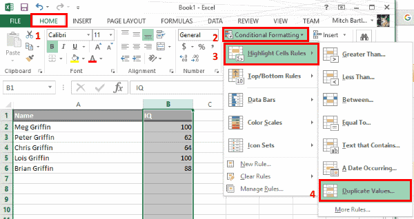 600×318 excel highlight duplicate unique cells from www.technipages.com
  624×444 highlight duplicate values excel teachexcelcom from www.teachexcel.com
  789×462 highlight duplicate values excel google sheets automate excel from www.automateexcel.com
 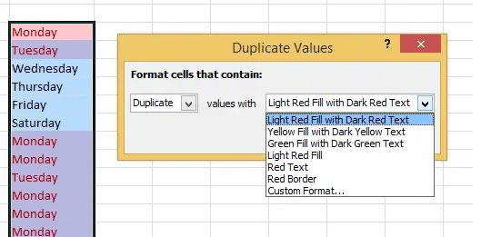 529×261 excel tip highlight duplicate values excel excel excel from howtoexcelatexcel.com
  970×456 highlight duplicate rows multiple columns excel from www.extendoffice.com
  396×191 highlighting duplicate values excel excel from blog.extrobe.co.uk
  420×242 highlight duplicates excel examples highlight duplicates from www.educba.com
  630×488 find highlight remove duplicates excel from www.exceldemy.com
  768×461 highlight duplicates microsoft excel from www.groovypost.com
  510×383 highlight duplicate values instance excel from www.extendoffice.com
 How To Highlight Duplicate Values In Excel was posted in November 15, 2025 at 1:07 pm. If you wanna have it as yours, please click the Pictures and you will go to click right mouse then Save Image As and Click Save and download the How To Highlight Duplicate Values In Excel Picture.. Don’t forget to share this picture with others via Facebook, Twitter, Pinterest or other social medias! we do hope you'll get inspired by ExcelKayra... Thanks again! If you have any DMCA issues on this post, please contact us!