How To Lock Rows And Columns In Excel For Scrolling
How To Lock Rows And Columns In Excel For Scrolling - There are a lot of affordable templates out there, but it can be easy to feel like a lot of the best cost a amount of money, require best special design template. Making the best template format choice is way to your template success. And if at this time you are looking for information and ideas regarding the How To Lock Rows And Columns In Excel For Scrolling then, you are in the perfect place. Get this How To Lock Rows And Columns In Excel For Scrolling for free here. We hope this post How To Lock Rows And Columns In Excel For Scrolling inspired you and help you what you are looking for.
Locking Rows and Columns in Excel: Freezing Panes for Enhanced Navigation
Excel spreadsheets can grow quite large, making it challenging to keep track of headers and key identifiers as you scroll through extensive datasets. Fortunately, Excel provides a powerful feature called “Freezing Panes” that allows you to lock specific rows and columns in place, ensuring they remain visible regardless of how far you scroll horizontally or vertically. This capability significantly improves navigation and data comprehension, especially when working with large spreadsheets.
Understanding Freezing Panes
Freezing panes essentially divides your worksheet into distinct sections. The rows and/or columns that you “freeze” remain stationary, while the rest of the worksheet scrolls beneath them. This means that crucial labels, headings, or reference data are always in view, providing context and preventing you from losing track of the information you’re working with.
How to Freeze Rows and Columns
Excel offers several options for freezing panes, each catering to different needs:
1. Freezing the Top Row
This is arguably the most common and simplest freezing option. It’s ideal when your column headers are located in the first row of your spreadsheet.
- Open your Excel spreadsheet.
- Navigate to the “View” tab on the Excel ribbon.
- In the “Window” group, click on the “Freeze Panes” dropdown menu.
- Select “Freeze Top Row”.
Now, as you scroll vertically down the spreadsheet, the top row will remain locked in place, ensuring your column headers are always visible.
2. Freezing the First Column
Similar to freezing the top row, this option is useful when your row identifiers or primary labels are located in the first column.
- Open your Excel spreadsheet.
- Navigate to the “View” tab on the Excel ribbon.
- In the “Window” group, click on the “Freeze Panes” dropdown menu.
- Select “Freeze First Column”.
As you scroll horizontally across the spreadsheet, the first column will remain stationary, keeping your row identifiers in sight.
3. Freezing Multiple Rows and Columns (Specific Panes)
This is the most flexible and powerful freezing option, allowing you to freeze any combination of rows and columns. This is particularly useful when you have multi-level headers or require both row and column labels to remain visible.
- Open your Excel spreadsheet.
- Select the cell below the row(s) and to the right of the column(s) that you want to freeze. This is a crucial step. For example, if you want to freeze the first two rows and the first column, you would select cell B3. Think of the selected cell as the “anchor” point for the freeze. Everything *above* and *to the left* of this cell will be frozen.
- Navigate to the “View” tab on the Excel ribbon.
- In the “Window” group, click on the “Freeze Panes” dropdown menu.
- Select “Freeze Panes” (the first option in the menu).
Now, scrolling vertically will keep the rows above the selected cell frozen, and scrolling horizontally will keep the columns to the left of the selected cell frozen.
Example: If you want to freeze rows 1 and 2 and columns A and B, you would select cell C3 before choosing the “Freeze Panes” option.
Unfreezing Panes
To remove the frozen panes and return your worksheet to its default scrolling behavior:
- Navigate to the “View” tab on the Excel ribbon.
- In the “Window” group, click on the “Freeze Panes” dropdown menu.
- Select “Unfreeze Panes”.
This will release all frozen rows and columns, allowing you to scroll freely throughout the entire worksheet.
Practical Applications and Benefits
Freezing panes offers numerous advantages, especially when working with large and complex spreadsheets:
- Improved Data Comprehension: By keeping headers and labels visible, you can easily understand the meaning and context of the data you’re viewing. This is crucial for accurate analysis and decision-making.
- Enhanced Navigation: Quickly navigate through large datasets without losing track of essential information. This saves time and reduces the risk of errors.
- Simplified Data Entry: When entering data into long rows or columns, frozen headers and labels provide constant guidance, ensuring accuracy and consistency.
- Effective Data Comparison: Compare data points across different rows or columns while keeping relevant identifiers in sight. This is particularly useful for identifying trends and patterns.
- Presentation-Ready Spreadsheets: Frozen panes make your spreadsheets more user-friendly and easier to present to others. Viewers can quickly grasp the content without needing to constantly scroll back and forth.
Tips and Considerations
- Plan Ahead: Before freezing panes, consider which rows and columns are most critical for maintaining context and understanding your data.
- Experiment: Try different freezing options to find the configuration that best suits your specific needs and the structure of your spreadsheet.
- Adjust as Needed: If the structure of your spreadsheet changes, don’t hesitate to unfreeze and re-freeze panes to adapt to the new layout.
- Be Mindful of Screen Size: On smaller screens, freezing too many rows or columns can significantly reduce the visible area of the scrollable region. Strike a balance between visibility and screen real estate.
- Alternative: Split Windows: For some tasks, the “Split” window feature (also found on the “View” tab) might offer a better solution than freezing panes. “Split” creates multiple independently scrollable views of the same worksheet.
Conclusion
Freezing panes is an indispensable tool for anyone who works with large Excel spreadsheets. By strategically locking rows and columns, you can significantly improve navigation, data comprehension, and overall productivity. Mastering this feature will empower you to work more efficiently and effectively with even the most complex datasets.
 624×374 freeze lock specific rows columns scrolling excel from www.teachexcel.com
 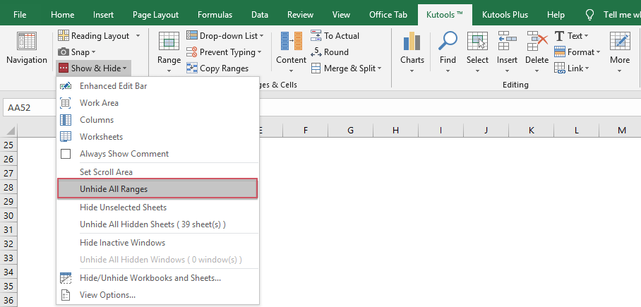 908×435 lock screen prevent scrolling excel worksheet from www.extendoffice.com
  700×400 turn scroll lock excel exceljet from exceljet.net
 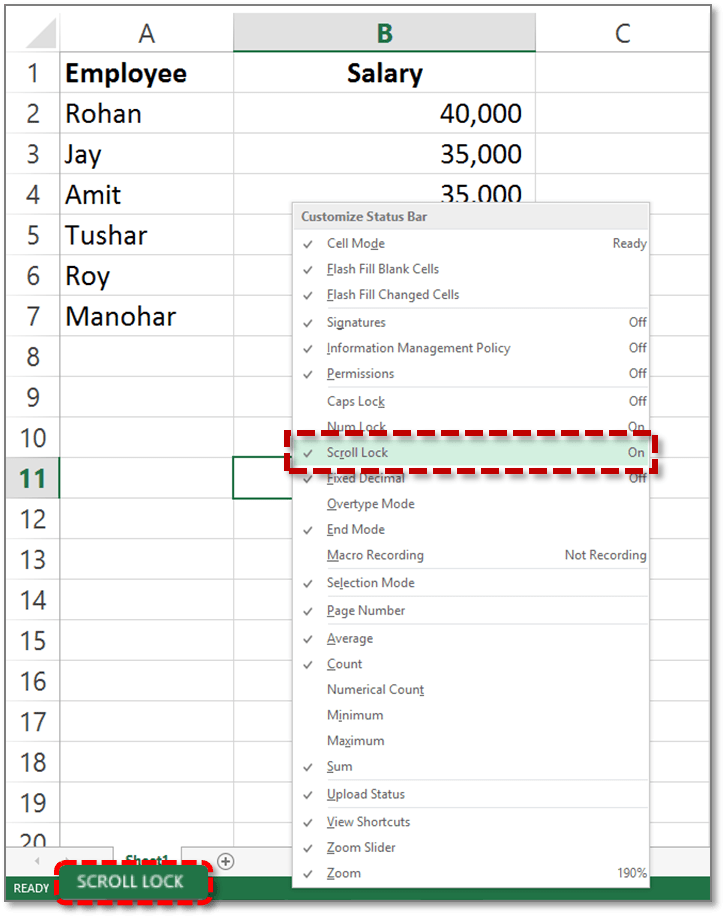 725×918 turn onoff scroll lock excel enabledisable scroll lock quickly from yodalearning.com
 How To Lock Rows And Columns In Excel For Scrolling was posted in September 29, 2025 at 11:01 am. If you wanna have it as yours, please click the Pictures and you will go to click right mouse then Save Image As and Click Save and download the How To Lock Rows And Columns In Excel For Scrolling Picture.. Don’t forget to share this picture with others via Facebook, Twitter, Pinterest or other social medias! we do hope you'll get inspired by ExcelKayra... Thanks again! If you have any DMCA issues on this post, please contact us!