Home » Excel Templates » How To Make A Checklist With Checkboxes In Excel

How To Make A Checklist With Checkboxes In Excel

Tuesday, February 10th 2026. | Excel Templates

How To Make A Checklist With Checkboxes In Excel - There are a lot of affordable templates out there, but it can be easy to feel like a lot of the best cost a amount of money, require best special design template. Making the best template format choice is way to your template success. And if at this time you are looking for information and ideas regarding the How To Make A Checklist With Checkboxes In Excel then, you are in the perfect place. Get this How To Make A Checklist With Checkboxes In Excel for free here. We hope this post How To Make A Checklist With Checkboxes In Excel inspired you and help you what you are looking for.

create checklist excel

“`html

Creating Checklists with Checkboxes in Excel

Excel is a powerful tool not just for data analysis, but also for organization and project management. One simple yet effective technique is using checklists with checkboxes. They are incredibly useful for tracking progress, managing tasks, and ensuring nothing gets missed. This guide will walk you through several methods to create dynamic and interactive checklists in Excel.

Method 1: Using the Developer Tab

The most straightforward method involves utilizing the Developer tab, which isn’t visible by default. You’ll need to enable it first.

Enabling the Developer Tab

Go to File > Options.
In the Excel Options dialog box, click on Customize Ribbon.
On the right-hand side, under the “Customize the Ribbon” section, find “Developer” in the list of Main Tabs.
Check the box next to “Developer” and click OK.

The Developer tab should now appear in your Excel ribbon.

Inserting Checkboxes

Navigate to the Developer tab.
In the “Controls” group, click Insert.
Under “Form Controls,” choose the Checkbox icon (the first icon in the top row).
Click and drag on your worksheet to draw the checkbox.
Right-click on the checkbox and select Edit Text. Remove the default text (e.g., “Check Box 1”) if you want the checkbox to appear without any label or with a different label next to it. You can also resize the checkbox as needed.
Repeat steps 3-5 to add more checkboxes to your list.

Linking Checkboxes to Cells

To make the checkboxes truly useful, you need to link them to cells. This allows you to track whether a checkbox is checked (TRUE) or unchecked (FALSE) in a cell. This link is what enables dynamic actions like conditional formatting or counting completed tasks.

Right-click on the checkbox you want to link.
Select Format Control.
In the “Format Control” dialog box, go to the Control tab.
In the “Cell link” box, click and select the cell you want to link the checkbox to. For instance, if the checkbox is in cell A2, you might link it to cell B2.
Click OK.
Repeat these steps for all your checkboxes, linking each to a different cell.

Now, when you check or uncheck a checkbox, the linked cell will display either TRUE or FALSE. You can then use these TRUE/FALSE values in formulas and conditional formatting.

Method 2: Using Wingdings Font (Alternative, Less Interactive)

This method provides a visual checklist but doesn’t offer the same interactivity as the Developer tab checkboxes. It relies on changing font characters to represent checked and unchecked boxes.

In a cell, type the character “o” (lowercase “o”). This will represent an unchecked box.
Select the cell.
In the Font dropdown (on the Home tab, in the Font group), choose Wingdings (or Wingdings 2 if ‘o’ doesn’t produce a box).
The “o” should transform into an empty square.
In an adjacent cell, type the character “p” (lowercase “p”).
Select the cell.
Change the font to Wingdings. The “p” should transform into a checked box (a square with a tick inside).
To create a list, copy the cell containing the empty square down your column.

This method is primarily visual. To mark a task as complete, you’d manually change the “o” to a “p”. It doesn’t provide a TRUE/FALSE value or integration with formulas.

Enhancing Your Checklists

Once you have your basic checklist, you can enhance it with features to make it more useful.

Conditional Formatting

Conditional formatting can visually highlight rows based on the checkbox status. For example, you can gray out or strikethrough a row when the corresponding checkbox is checked.

Select the entire range of cells containing your task descriptions and any other associated data (e.g., from column A to column C if your tasks are in column A and your checkboxes are linked to column B, and column C contains additional information).
Go to the Home tab.
In the “Styles” group, click on Conditional Formatting.
Select New Rule…
Choose “Use a formula to determine which cells to format.”
In the formula box, enter a formula that references the linked cell for the first checkbox in your selected range. For example, if your selected range starts in row 2 and the checkboxes are linked to column B, enter the formula =$B2=TRUE. The dollar sign ($) before the column letter ensures that the column remains fixed when the formatting is applied to the entire range.
Click the Format… button.
Choose the formatting you want to apply when the checkbox is checked (e.g., a gray fill color, strikethrough font).
Click OK on the Format Cells dialog and then OK on the New Formatting Rule dialog.

Now, when you check a checkbox, the corresponding row will be formatted according to the rule you defined.

Counting Completed Tasks

You can use the COUNTIF function to automatically count how many tasks have been completed.

In a cell (e.g., D2), enter the formula =COUNTIF(B2:B10,TRUE). Replace `B2:B10` with the actual range of cells that your checkboxes are linked to.
This formula will count the number of cells in the specified range that contain the value TRUE.

This cell will now display the number of completed tasks.

Creating a Completion Percentage

You can calculate the percentage of tasks that are completed using the COUNTIF function and the total number of tasks.

In a cell (e.g., E2), enter the formula =(COUNTIF(B2:B10,TRUE)/COUNTA(A2:A10))*100. Replace `B2:B10` with the range of cells linked to checkboxes, and `A2:A10` with the range of task descriptions.
This formula divides the number of TRUE values (completed tasks) by the total number of tasks and multiplies by 100 to get the percentage.
Format the cell as a percentage by clicking the “%” button on the Home tab (in the Number group).

This cell will now display the percentage of tasks completed.

Considerations

Protecting your Sheet: Consider protecting your worksheet (Review tab > Protect Sheet) to prevent accidental changes to the formulas and checkbox links. You can allow users to interact with the checkboxes while protecting the rest of the sheet.
Large Lists: For very large lists, using named ranges can make formulas easier to understand and maintain.
Data Validation: Consider using Data Validation to ensure that the task descriptions are consistent and avoid typos.

Creating checklists with checkboxes in Excel can significantly improve your organizational skills and project management capabilities. By using the Developer tab and linking checkboxes to cells, you can create dynamic and interactive checklists that automatically update based on your progress. The added features of conditional formatting and task counting provide even more value and insights into your workflow.

“`

541×347 checklist excel create checklist excel examples from www.educba.com

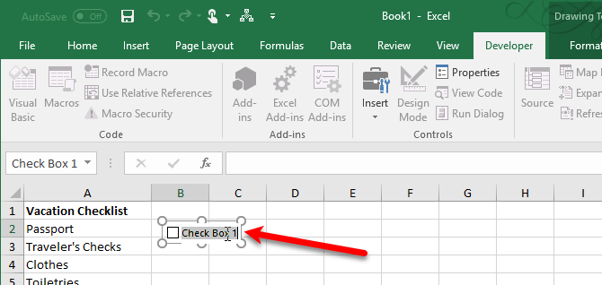670×318 checklist excel edrawmax from www.edrawmax.com

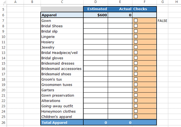624×436 checkboxes create checklist template excel from www.exceltip.com

452×398 insert checkbox excel from www.repairmsexcel.com

588×576 create checklist excel from www.dotnetheaven.com

How To Make A Checklist With Checkboxes In Excel was posted in February 10, 2026 at 7:52 pm. If you wanna have it as yours, please click the Pictures and you will go to click right mouse then Save Image As and Click Save and download the How To Make A Checklist With Checkboxes In Excel Picture.. Don’t forget to share this picture with others via Facebook, Twitter, Pinterest or other social medias! we do hope you'll get inspired by ExcelKayra... Thanks again! If you have any DMCA issues on this post, please contact us!