How To Use Data Validation With Formulas In Excel
How To Use Data Validation With Formulas In Excel - There are a lot of affordable templates out there, but it can be easy to feel like a lot of the best cost a amount of money, require best special design template. Making the best template format choice is way to your template success. And if at this time you are looking for information and ideas regarding the How To Use Data Validation With Formulas In Excel then, you are in the perfect place. Get this How To Use Data Validation With Formulas In Excel for free here. We hope this post How To Use Data Validation With Formulas In Excel inspired you and help you what you are looking for.
Using Data Validation with Formulas in Excel
Data validation in Excel is a powerful feature that allows you to control the type of data that users can enter into a cell. While basic data validation rules like restricting entries to numbers, dates, or a predefined list are helpful, combining data validation with formulas unlocks a new level of flexibility and precision. This allows you to create dynamic and intelligent validation rules that adapt to changing data and complex requirements.
Why Use Formulas in Data Validation?
The primary advantage of using formulas in data validation is that it makes your validation rules dynamic. Instead of being limited to static lists or simple numeric ranges, you can base your validation criteria on other cells, calculated values, or even external data sources. This opens the door to several advanced scenarios:
- Conditional Validation: You can change the validation rules based on the value in another cell. For example, if a cell contains “Yes,” you might require a date to be entered in the validated cell; otherwise, the cell should remain blank.
- Dynamic Lists: You can create a list of valid entries that automatically updates based on data elsewhere in the spreadsheet. This is useful for managing inventory lists or customer names.
- Complex Constraints: You can implement validation rules that involve multiple criteria and complex calculations. For example, you might require that a number be within a certain percentage of another number.
- Preventing Circular References: Data validation, when used carefully, can prevent circular references from happening, improving workbook stability.
How to Implement Data Validation with Formulas
Here’s a step-by-step guide to using formulas in data validation:
- Select the Cell(s) to Validate: Begin by selecting the cell or range of cells where you want to apply the data validation rule.
- Open the Data Validation Dialog: Go to the “Data” tab on the Excel ribbon and click on “Data Validation.” This will open the Data Validation dialog box.
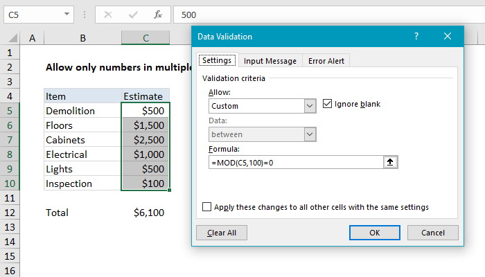
- Choose “Custom” as the Validation Criteria: In the Data Validation dialog box, on the “Settings” tab, select “Custom” from the “Allow” dropdown menu. This is where you’ll enter your formula.
- Enter Your Formula: In the “Formula” box, type your formula. The formula must evaluate to either TRUE or FALSE. If the formula evaluates to TRUE for a given cell value, the entry is considered valid; otherwise, it’s considered invalid.
- Customize the Error Alert (Optional): Go to the “Error Alert” tab to customize the error message that is displayed when a user enters an invalid value. You can choose the style of the error alert (Stop, Warning, or Information) and enter a custom title and error message. A “Stop” style will prevent the user from entering the data. A “Warning” will allow the user to continue with the input if they wish. Information is similar to warning, but less assertive.
- Customize the Input Message (Optional): Go to the “Input Message” tab to display a message when the user selects the validated cell. This can be helpful to guide the user on what data is expected. You can specify a title and message.
- Click “OK”: Click the “OK” button to apply the data validation rule.
Examples of Data Validation Formulas
Here are several examples of how to use formulas in data validation, along with explanations:
1. Restricting Input to Numbers Greater Than a Value in Another Cell
Scenario: You want to ensure that a cell (e.g., A1) only accepts numbers that are greater than the value in cell B1.
Formula: =A1>B1
Explanation: This formula compares the value entered in cell A1 with the value in cell B1. If the value in A1 is greater than the value in B1, the formula returns TRUE, and the entry is valid. Otherwise, it returns FALSE, and the entry is rejected.
2. Ensuring a Date is Within a Specific Range Relative to Another Date
Scenario: You want to ensure that a date entered in a cell (e.g., C1) is within 30 days of the date in cell D1.
Formula: =AND(C1>=D1-30, C1<=D1+30)
Explanation: This formula uses the AND function to combine two conditions. The first condition (C1>=D1-30) checks if the date in C1 is greater than or equal to the date in D1 minus 30 days. The second condition (C1<=D1+30) checks if the date in C1 is less than or equal to the date in D1 plus 30 days. Both conditions must be true for the formula to return TRUE and allow the entry.
3. Validating Email Addresses
Scenario: You want to ensure that the text entered in a cell looks like a valid email address.
Formula: =AND(ISNUMBER(FIND("@",A1)),ISNUMBER(FIND(".",A1)),NOT(ISBLANK(A1)))
Explanation: This formula is not foolproof (it doesn't validate the domain's existence), but it's a good starting point. The formula checks for three conditions:
- The
FIND("@",A1)function searches for the "@" symbol in cell A1.ISNUMBERchecks if theFINDfunction returns a number (meaning the "@" symbol was found). - The
FIND(".",A1)function searches for the "." symbol in cell A1.ISNUMBERchecks if theFINDfunction returns a number (meaning the "." symbol was found). - The
NOT(ISBLANK(A1))function checks if cell A1 is not blank.
All three conditions must be true for the entry to be considered a valid email address (or at least, to contain the basic structure of one).
4. Creating a Dependent List
Scenario: You want to create a list of options that changes based on the selection made in another cell (for example, selecting a country and then only showing cities in that country). This requires named ranges and the INDIRECT function.
Steps:
- Set up your data: In one area of your sheet, list the categories (e.g., Countries) in the first column (e.g., A1:A3 – USA, Canada, UK). In adjacent columns, list the options for each category (e.g., B1:B3 – New York, Los Angeles, Chicago for USA; C1:C3 – Toronto, Montreal, Vancouver for Canada).
- Create Named Ranges: Select each range of options for each category (e.g., B1:B3). Go to the "Formulas" tab and click "Define Name." Enter the *exact same name* as the corresponding category in column A (e.g., name B1:B3 as "USA"). Repeat for each country. It's crucial the named ranges match the entries in the "country" selection cell *exactly*. You might also want to name the 'country' column as "country_list".
- Apply Data Validation to the "Country" Cell: Select the cell where you want the country selection. Go to Data Validation, choose "List," and enter
=country_listas the source. - Apply Data Validation to the "City" Cell: Select the cell where you want the city selection. Go to Data Validation, choose "List," and enter
=INDIRECT(A1)as the source (assuming the country selection is in cell A1).
Explanation: The INDIRECT function takes the text value in cell A1 (the selected country) and treats it as a named range. Since you've named the ranges containing the city options with the corresponding country names, INDIRECT dynamically retrieves the correct list of cities for the selected country.
5. Preventing Duplicate Entries in a Column
Scenario: You want to ensure that entries in a column are unique.
Formula: =COUNTIF($A:$A,A1)=1 (applied to column A)
Explanation: This formula uses the COUNTIF function to count the number of times the value in cell A1 appears in the entire column A. If the count is equal to 1 (meaning the value only appears once), the formula returns TRUE, and the entry is valid. If the count is greater than 1 (meaning the value is a duplicate), the formula returns FALSE, and the entry is rejected. The $A:$A ensures that the COUNTIF function always looks at the entire column A, even when the formula is applied to other cells in the column. This is critical for accurate duplicate checking.
Tips and Considerations
- Absolute vs. Relative References: Pay close attention to whether you need to use absolute (
$) or relative references in your formulas. Absolute references prevent the cell references from changing when the data validation rule is applied to multiple cells. Relative references change appropriately as the validation is applied to more than one cell. - Testing: Thoroughly test your data validation rules with different scenarios and edge cases to ensure they work as expected.
- Error Messages: Customize the error messages to be clear and helpful to users. Explain why the entry is invalid and what is expected.
- Formula Complexity: While formulas can be powerful, avoid creating overly complex formulas that are difficult to understand and maintain. Break down complex validation requirements into smaller, more manageable steps if possible.
- Performance: If you have a large spreadsheet with many data validation rules using complex formulas, it can impact performance. Consider optimizing your formulas or using alternative approaches if necessary.
- Circular References: Be cautious when using data validation to modify cells that influence the validation itself. This can lead to circular reference errors and unpredictable behavior. Carefully design your validation rules to avoid these issues.
Conclusion
Using data validation with formulas in Excel provides a powerful and flexible way to control data entry and ensure data quality. By understanding the principles and techniques outlined in this guide, you can create sophisticated validation rules that adapt to changing data and complex requirements, making your spreadsheets more robust and user-friendly.
 700×400 data validation formula examples exceljet from exceljet.net
 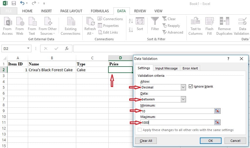 853×507 learn data validation techniques excel excelbuddycom from excelbuddy.com
  800×600 data validation excel customguide from www.customguide.com
  1333×1000 understanding excel data validation rockets marketing from 500rockets.io
  600×315 data validation excel step step tutorial from www.excel-easy.com
  408×484 data validation excel custom validation rules formulas from www.ablebits.com
  641×383 data validation excel examples create data validation from www.educba.com
 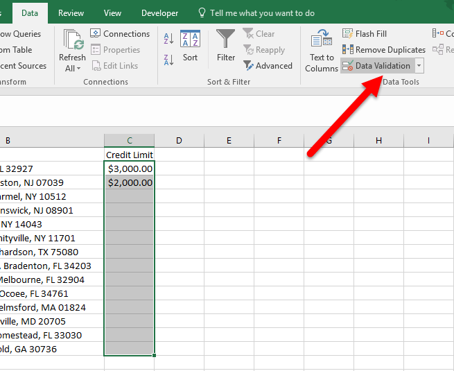 655×535 learn excel data validation cells theapptimes from theapptimes.com
 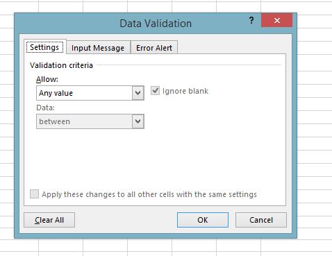 478×369 data validation excel from www.simplilearn.com
  953×528 ways data validation excel from gyankosh.net
 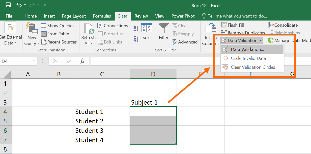 1255×623 create data validation microsoft excel webnots from www.webnots.com
 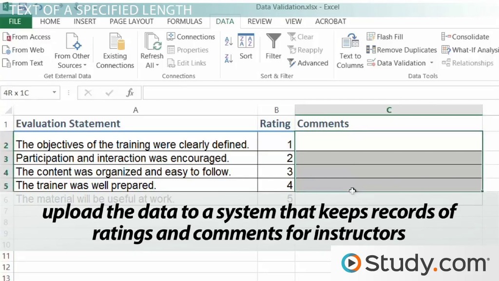 0 x 0 data validation excel lesson studycom from study.com
 How To Use Data Validation With Formulas In Excel was posted in October 2, 2025 at 4:42 am. If you wanna have it as yours, please click the Pictures and you will go to click right mouse then Save Image As and Click Save and download the How To Use Data Validation With Formulas In Excel Picture.. Don’t forget to share this picture with others via Facebook, Twitter, Pinterest or other social medias! we do hope you'll get inspired by ExcelKayra... Thanks again! If you have any DMCA issues on this post, please contact us!