How To Use Indirect Function In Excel For Dynamic Data
How To Use Indirect Function In Excel For Dynamic Data - There are a lot of affordable templates out there, but it can be easy to feel like a lot of the best cost a amount of money, require best special design template. Making the best template format choice is way to your template success. And if at this time you are looking for information and ideas regarding the How To Use Indirect Function In Excel For Dynamic Data then, you are in the perfect place. Get this How To Use Indirect Function In Excel For Dynamic Data for free here. We hope this post How To Use Indirect Function In Excel For Dynamic Data inspired you and help you what you are looking for.
Using the INDIRECT Function in Excel for Dynamic Data
The INDIRECT function in Excel is a powerful tool that allows you to create dynamic references to cells, ranges, or even other worksheets. Instead of directly referencing a cell (e.g., A1), INDIRECT lets you specify the cell reference as a text string, enabling you to build references that change based on the values in other cells. This capability opens up a wide range of possibilities for creating flexible and interactive spreadsheets.
Understanding the Syntax
The syntax of the INDIRECT function is straightforward:
=INDIRECT(ref_text, [a1])- ref_text: This is the text string that represents the cell or range reference you want to retrieve. It can be a hardcoded text string (e.g., “A1”) or a formula that generates a text string representing the reference.
- [a1]: This is an optional argument that specifies the referencing style. It can be either:
- TRUE (or omitted): Indicates A1-style referencing (e.g., A1, B2, C3). This is the default.
- FALSE: Indicates R1C1-style referencing (e.g., R1C1, R2C3).
Basic Usage: Referencing a Cell
The simplest use of INDIRECT is to retrieve the value of a cell specified as a text string.
Example:
- In cell A1, enter the value “100”.
- In cell B1, enter the text string “A1”.
- In cell C1, enter the formula: `=INDIRECT(B1)`
Cell C1 will display the value 100, because INDIRECT(B1) evaluates to INDIRECT(“A1”), which then retrieves the value from cell A1.
Dynamic Cell References
The real power of INDIRECT comes from its ability to create dynamic references based on the values in other cells. This allows your formulas to adapt to changing data or user inputs.
Example: Creating a Dynamic Column Selector
- In row 1, enter column headers: “Name” in A1, “Age” in B1, “City” in C1.
- In column A, rows 2-4, enter names: “Alice”, “Bob”, “Charlie”.
- In column B, rows 2-4, enter ages: 25, 30, 28.
- In column C, rows 2-4, enter cities: “New York”, “London”, “Paris”.
- In cell E1, create a dropdown list using Data Validation that allows the user to select a column header: “Name”, “Age”, or “City”. Go to Data > Data Validation > Allow: List > Source: A1:C1
- In cell E2, enter the formula: `=INDIRECT(ADDRESS(ROW(),MATCH(E1,A1:C1,0)))`
- Copy the formula in E2 down to cells E3 and E4.
Explanation:
- E1: Contains the selected column header (“Name”, “Age”, or “City”).
- MATCH(E1, A1:C1, 0): This function finds the position of the selected column header within the range A1:C1. For example, if E1 is “Age”, MATCH returns 2.
- ROW(): Returns the current row number. In E2, it returns 2; in E3, it returns 3; and so on.
- ADDRESS(ROW(), MATCH(E1,A1:C1,0)): This function constructs a cell address as a text string. It takes the row number (from ROW()) and the column number (from MATCH) as arguments. For example, if E1 is “Age” and you are in cell E2, ADDRESS returns “B2”.
- INDIRECT(ADDRESS(…)): Finally, the INDIRECT function takes the cell address string generated by ADDRESS and retrieves the value from that cell. In this case, it would retrieve the age for the corresponding person (Alice, Bob, or Charlie).
Now, when you change the selected column header in cell E1, the values in cells E2:E4 will dynamically update to display the corresponding data from the selected column.
Referencing Other Worksheets
INDIRECT can also be used to reference cells or ranges in other worksheets. The sheet name must be included in the `ref_text`.
Example: Retrieving a Value from Another Sheet
- Create two worksheets: “Sheet1” and “Sheet2”.
- In cell A1 of “Sheet2”, enter the value “200”.
- In cell A1 of “Sheet1”, enter the formula: `=INDIRECT(“‘Sheet2’!A1”)`
Cell A1 of “Sheet1” will display the value 200, which is the value in cell A1 of “Sheet2”. Note the single quotes around the sheet name. These are necessary if the sheet name contains spaces or special characters.
Example: Dynamic Sheet Selection
- Create three worksheets: “January”, “February”, and “March”.
- In cell A1 of each sheet, enter a value specific to that month (e.g., “10” in January, “20” in February, “30” in March).
- In cell A1 of a new sheet (e.g., “Summary”), create a dropdown list using Data Validation with the months “January”, “February”, and “March” as the list source.
- In cell A2 of the “Summary” sheet, enter the formula: `=INDIRECT(“‘”&A1&”‘!A1”)`
When you select a month from the dropdown list in cell A1 of the “Summary” sheet, cell A2 will dynamically display the value from cell A1 of the corresponding month’s sheet.
Using R1C1 Referencing Style
While A1 referencing is more common, INDIRECT can also work with R1C1 referencing. Remember to set the `a1` argument to FALSE.
Example:
- In cell A1, enter the value “300”.
- In cell B1, enter the text string “R1C1”.
- In cell C1, enter the formula: `=INDIRECT(B1, FALSE)`
Cell C1 will display the value 300 because R1C1 refers to the cell in the first row and first column (A1).
Example: Retrieving Value from the Cell Directly Below
- In A1 Enter Header “Name”
- In A2 Enter “John”
- In B1 Enter “=INDIRECT(“”R[1]C[-1]””,FALSE)”
B1 will display “John”. R[1] refers to one row down and C[-1] refers to one column to the left, from B1.
Common Errors and Troubleshooting
- #REF! Error: This error usually indicates that the `ref_text` argument is invalid or refers to a non-existent cell or range. Double-check the spelling and syntax of the text string, especially when constructing it dynamically. Also, ensure that the referenced sheet exists.
- Circular Reference Error: Be careful not to create circular references with INDIRECT. A circular reference occurs when a formula directly or indirectly refers to its own cell.
- Volatile Function: INDIRECT is a volatile function, which means it recalculates whenever any cell in the worksheet changes, even if the cells it references are not affected. This can slow down large or complex spreadsheets. Use INDIRECT judiciously. Consider alternative solutions if performance becomes an issue.
- Sheet Name Errors: Remember to enclose sheet names in single quotes if they contain spaces or special characters.
Alternatives to INDIRECT
While INDIRECT is powerful, it’s often a good idea to consider alternative approaches, especially if performance is a concern.
- INDEX and MATCH: These functions can often achieve the same results as INDIRECT, but without the volatility. They are particularly useful for looking up values in tables.
- OFFSET: Similar to INDEX and MATCH, OFFSET can return a range of cells relative to a starting point.
- Named Ranges: Defining named ranges can make your formulas more readable and maintainable, and can sometimes eliminate the need for dynamic references.
Conclusion
The INDIRECT function is a valuable tool for creating dynamic and flexible spreadsheets in Excel. It allows you to build cell references programmatically, making your formulas adaptable to changing data and user inputs. While it’s important to be aware of its volatility and potential performance implications, mastering INDIRECT can significantly enhance your spreadsheet modeling capabilities. Understanding its syntax, potential errors, and alternative approaches will allow you to leverage its power effectively.
 1301×586 excel indirect function excelfind from excelfind.com
  572×428 indirect function excel examples from www.exceldemy.com
 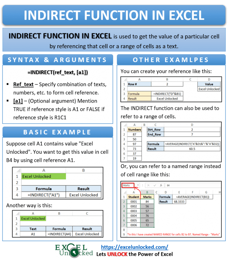 768×881 indirect function excel values reference excel unlocked from excelunlocked.com
  465×202 excel indirect function excel vba from www.exceldome.com
  400×215 indirect dynamically reference cell excel aj from www.articlejobber.com
  1220×525 excel indirect function step step from careerfoundry.com
  944×648 excel indirect function formula details video examples from www.someka.net
  1405×527 excel indirect function complete guide from excelsirji.com
  1280×720 excel indirect function earn excel from earnandexcel.com
 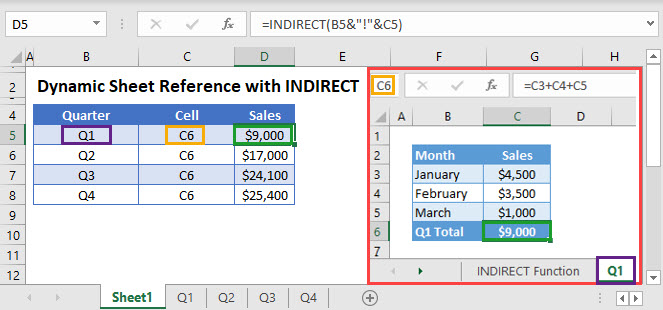 663×310 dynamic sheet reference indirect excel google sheets from www.automateexcel.com
 :max_bytes(150000):strip_icc()/excel-indirect-function-580bb7145f9b58564cf69f6f.jpg) 1153×661 learning excel indirect function from www.lifewire.com
1153×661 learning excel indirect function from www.lifewire.com  386×187 excel indirect function training hub from www.myonlinetraininghub.com
  480×360 indirect function excel knowledge sharing from bajidotnet.wordpress.com
  622×538 excel indirect function examples pakaccountantscom from pakaccountants.com
 How To Use Indirect Function In Excel For Dynamic Data was posted in October 16, 2025 at 3:51 pm. If you wanna have it as yours, please click the Pictures and you will go to click right mouse then Save Image As and Click Save and download the How To Use Indirect Function In Excel For Dynamic Data Picture.. Don’t forget to share this picture with others via Facebook, Twitter, Pinterest or other social medias! we do hope you'll get inspired by ExcelKayra... Thanks again! If you have any DMCA issues on this post, please contact us!