How To Use Indirect Function In Excel For Flexible Referencing
How To Use Indirect Function In Excel For Flexible Referencing - There are a lot of affordable templates out there, but it can be easy to feel like a lot of the best cost a amount of money, require best special design template. Making the best template format choice is way to your template success. And if at this time you are looking for information and ideas regarding the How To Use Indirect Function In Excel For Flexible Referencing then, you are in the perfect place. Get this How To Use Indirect Function In Excel For Flexible Referencing for free here. We hope this post How To Use Indirect Function In Excel For Flexible Referencing inspired you and help you what you are looking for.
“`html
Using the INDIRECT Function in Excel for Flexible Referencing
The INDIRECT function in Excel is a powerful tool that allows you to create flexible and dynamic references to cells or ranges. Instead of directly specifying the cell or range address, you provide a text string that evaluates to that address. This seemingly simple feature unlocks a wide range of possibilities for building more robust, adaptable, and user-friendly spreadsheets.
Understanding the Basics
The syntax of the INDIRECT function is:
=INDIRECT(ref_text, [a1])
- ref_text: This is a text string that represents the cell or range you want to refer to. This string can be entered directly (e.g., “A1”) or built dynamically using other functions and cell values.
- [a1]: This is an optional argument that specifies the referencing style of
ref_text.- If set to TRUE (or omitted),
ref_textis interpreted as an A1-style reference (e.g., “A1”, “B2:C10”). - If set to FALSE,
ref_textis interpreted as an R1C1-style reference (e.g., “R1C1”, “R2C3:R10C4”). R1C1 references use row and column numbers (e.g., R1C1 is row 1, column 1, which is equivalent to A1).
- If set to TRUE (or omitted),
In its simplest form, =INDIRECT("A1") returns the value of cell A1. While this simple example doesn’t showcase its power, it demonstrates the core concept: the function evaluates the text string “A1” to determine the cell to reference.
Key Applications and Examples
1. Dynamic Sheet Referencing
One of the most common uses of INDIRECT is to dynamically refer to different worksheets. Imagine you have monthly sales data on separate sheets named “January”, “February”, “March”, and so on. You can create a formula that pulls data from the appropriate sheet based on a cell containing the month name.
Example:
- Cell A1: Contains the text “January” (or “February”, etc.)
- Formula in B1:
=INDIRECT("'"&A1&"'!B2")
Explanation:
A1provides the sheet name."'"&A1&"'"adds single quotes around the sheet name. This is necessary if the sheet name contains spaces or special characters. Excel requires that sheet names with spaces be enclosed in single quotes when referred to in formulas."'"&A1&"'!B2"concatenates the sheet name with the cell reference “B2”. The exclamation point (!) separates the sheet name from the cell reference.INDIRECT("'"&A1&"'!B2")evaluates the resulting string (e.g., “‘January’!B2”) and returns the value from cell B2 on the “January” sheet.
By changing the value in cell A1, you can instantly switch the formula to retrieve data from different sheets without modifying the formula itself.
2. Creating Dynamic Named Ranges
Named ranges make your formulas more readable and maintainable. INDIRECT allows you to create named ranges that automatically adjust their size based on data changes.
Example:
- Assume your data starts in cell A1 and extends down the column.
- Assume cell B1 contains a formula that calculates the last row with data (e.g.,
=COUNTA(A:A)). - Go to Formulas > Define Name.
- In the “Name” field, enter a name for your dynamic range (e.g., “MyData”).
- In the “Refers to” field, enter the following formula:
=INDIRECT("A1:A"&B1)
Explanation:
B1contains the number of rows with data."A1:A"&B1concatenates the start of the range (“A1:A”) with the row number from B1. For example, if B1 contains “10”, the resulting string would be “A1:A10”.INDIRECT("A1:A"&B1)converts the text string “A1:A10” (or whatever the calculated range is) into an actual range that can be used in other formulas.
Now, the named range “MyData” will automatically expand or contract as you add or remove data in column A. You can then use “MyData” in formulas like =SUM(MyData) without needing to manually update the range reference.
3. Retrieving Values from Tables Based on Headers
When working with structured data in tables, you can use INDIRECT to retrieve values based on column headers.
Example:
- Assume you have a table with headers in row 1 (e.g., “Name”, “City”, “Sales”).
- Assume cell A2 contains the name “John”.
- Assume cell B1 contains the header you want to search for (e.g., “Sales”).
- The following formula in C2 will retrieve John’s sales figure:
=INDIRECT(ADDRESS(ROW(A2),COLUMN(INDEX(1:1,MATCH(B1,1:1,0)))))
Explanation (from the inside out):
MATCH(B1,1:1,0)finds the column number where the value in B1 (e.g., “Sales”) appears in row 1 (the headers).INDEX(1:1,MATCH(B1,1:1,0))returns the cell in row 1 where “Sales” is found (e.g., C1). This part is technically redundant, but serves to show the lookup in isolation.COLUMN(INDEX(1:1,MATCH(B1,1:1,0)))gets the column number of the cell found by theINDEXfunction (e.g., 3, since “Sales” is in column C).ROW(A2)gets the row number of cell A2 (e.g., 2).ADDRESS(ROW(A2),COLUMN(INDEX(1:1,MATCH(B1,1:1,0))))creates a cell address string using the row and column numbers obtained (e.g., “C2”).INDIRECT(ADDRESS(ROW(A2),COLUMN(INDEX(1:1,MATCH(B1,1:1,0)))))evaluates the address string “C2” and returns the value from cell C2 (John’s sales figure).
If you change the header in cell B1 (e.g., to “City”), the formula will automatically retrieve John’s city from the table.
This example can be simplified with =INDEX(A:Z,ROW(A2),MATCH(B1,1:1,0)) which doesn’t require INDIRECT, but the original example highlights a complex use case where the address might need to be constructed from several different pieces of information, making the INDIRECT approach very useful.
4. Working with R1C1 Referencing
While less common, using R1C1 referencing with INDIRECT can be useful for creating formulas that are relative to the cell containing the formula.
Example:
If you want to retrieve the value from the cell one row above and two columns to the left of the current cell, you can use the following formula:
=INDIRECT("R[-1]C[-2]", FALSE)
Explanation:
"R[-1]C[-2]"is the R1C1 reference.R[-1]means one row above the current cell, andC[-2]means two columns to the left of the current cell.FALSEtells INDIRECT to interpretref_textas an R1C1 reference.
Cautions and Considerations
- Volatility: INDIRECT is a volatile function. This means that Excel recalculates the formula every time any cell in the workbook changes, even if the INDIRECT formula is not directly related to the changed cell. Excessive use of INDIRECT can significantly slow down your spreadsheet. Consider alternative solutions like INDEX/MATCH or OFFSET if performance becomes an issue.
- Error Handling: If the
ref_textdoes not evaluate to a valid cell or range address, INDIRECT will return a#REF!error. Use IFERROR to handle potential errors gracefully. For example:=IFERROR(INDIRECT("'"&A1&"'!B2"), "Sheet not found"). - Readability: Complex INDIRECT formulas can be difficult to understand and debug. Use comments and descriptive cell names to improve readability.
- Circular References: Be careful to avoid creating circular references when using INDIRECT. A circular reference occurs when a formula refers to itself, either directly or indirectly.
Conclusion
The INDIRECT function is a powerful tool for creating flexible and dynamic references in Excel. While it should be used judiciously due to its volatility, it opens up possibilities for building sophisticated spreadsheets that can adapt to changing data and user input. By understanding its syntax and applications, you can leverage INDIRECT to create more robust and user-friendly solutions.
“`
 934×642 indirect function excel excelbuddycom from excelbuddy.com
  1301×586 excel indirect function excelfind from excelfind.com
 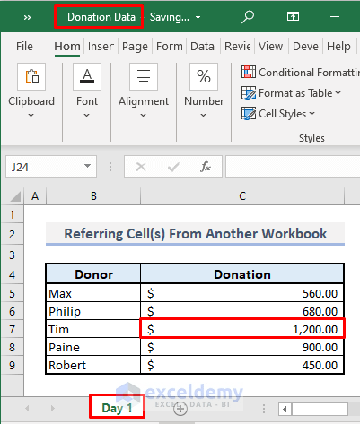 401×473 indirect function excel examples from www.exceldemy.com
  909×1043 indirect function excel values reference excel unlocked from excelunlocked.com
 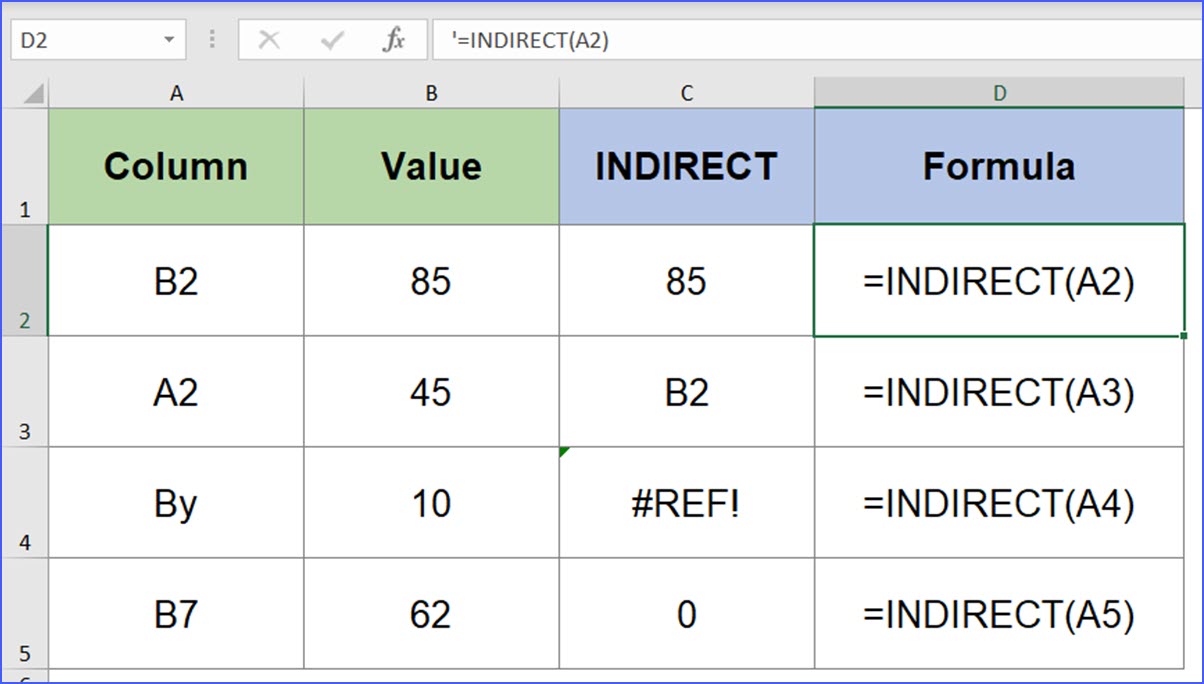 1204×684 indirect function excelnotes from excelnotes.com
 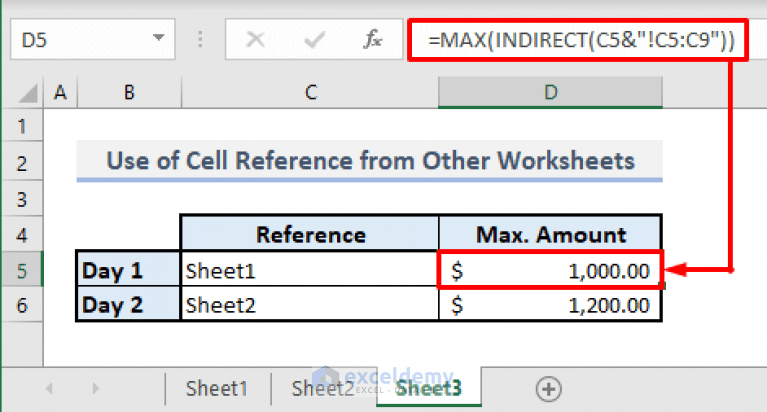 767×412 indirect function excel suitable instances from www.exceldemy.com
  474×338 excel indirect function complete guide from excelsirji.com
  1280×720 excel indirect function earn excel from earnandexcel.com
  720×376 excel indirect function goskills from www.goskills.com
 :max_bytes(150000):strip_icc()/excel-indirect-function-580bb7145f9b58564cf69f6f.jpg) 1153×661 learning excel indirect function from www.lifewire.com
1153×661 learning excel indirect function from www.lifewire.com 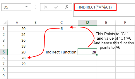 461×269 excel indirect function from www.exceltrick.com
 How To Use Indirect Function In Excel For Flexible Referencing was posted in August 6, 2025 at 6:13 am. If you wanna have it as yours, please click the Pictures and you will go to click right mouse then Save Image As and Click Save and download the How To Use Indirect Function In Excel For Flexible Referencing Picture.. Don’t forget to share this picture with others via Facebook, Twitter, Pinterest or other social medias! we do hope you'll get inspired by ExcelKayra... Thanks again! If you have any DMCA issues on this post, please contact us!