How To Use Pivot Table Slicers To Filter Data In Excel
How To Use Pivot Table Slicers To Filter Data In Excel - There are a lot of affordable templates out there, but it can be easy to feel like a lot of the best cost a amount of money, require best special design template. Making the best template format choice is way to your template success. And if at this time you are looking for information and ideas regarding the How To Use Pivot Table Slicers To Filter Data In Excel then, you are in the perfect place. Get this How To Use Pivot Table Slicers To Filter Data In Excel for free here. We hope this post How To Use Pivot Table Slicers To Filter Data In Excel inspired you and help you what you are looking for.
Using Pivot Table Slicers in Excel for Data Filtering
Pivot tables are powerful tools in Excel for summarizing and analyzing large datasets. They allow you to quickly extract meaningful insights by aggregating data based on different categories. However, sometimes you need more than just a summary; you need to dynamically filter the data to focus on specific subsets. This is where slicers come in. Slicers are visual filters that make it easy to interact with your pivot table and quickly refine the data displayed.
What are Slicers?
Slicers are interactive controls that provide a quick and easy way to filter pivot table data. They present a set of buttons representing the unique values in a field, and clicking a button filters the pivot table to show only the rows that match that value. Think of them as user-friendly replacements for traditional filter dropdowns, offering a more intuitive and visually appealing filtering experience.
Benefits of Using Slicers
Using slicers to filter data in pivot tables offers several advantages:
- Ease of Use: Slicers are extremely user-friendly. Clicking a button is much easier and faster than opening a filter dropdown and selecting values.
- Visual Clarity: Slicers provide a clear overview of available filter options. You can immediately see which values you can filter by, and which filters are currently active.
- Multiple Filter Application: You can easily apply multiple filters simultaneously by selecting multiple buttons on a single slicer or by using multiple slicers connected to the same pivot table.
- Dynamic Filtering: Changes made to slicers are instantly reflected in the pivot table, allowing for real-time exploration of data.
- Enhanced Presentation: Slicers can improve the visual appeal of your spreadsheets and dashboards, making them more engaging and easier to understand.
- Connectivity to Multiple Pivot Tables: A single slicer can control multiple pivot tables simultaneously, enabling synchronized filtering across different views of the same data.
How to Insert Slicers
Here’s how to insert slicers for your pivot table:
- Select the Pivot Table: Click anywhere within your pivot table to activate it. This will make the “PivotTable Analyze” (or “Options” in older Excel versions) tab appear in the Excel ribbon.
- Go to the “Insert Slicer” Option: In the “PivotTable Analyze” tab, locate the “Filter” group. Click on the “Insert Slicer” button.
- Choose the Fields for Slicers: The “Insert Slicers” dialog box will appear, listing all the fields in your pivot table source data. Check the boxes next to the fields you want to create slicers for. These fields should be those that you commonly use for filtering your data.
- Click “OK”: After selecting the desired fields, click “OK”. Excel will create a separate slicer for each selected field.
Using Slicers to Filter Data
Once you’ve inserted slicers, you can start using them to filter your pivot table:
- Single Selection: To filter the pivot table to show only data matching a specific value, simply click on the corresponding button in the slicer. The selected button will typically be highlighted (often in blue), indicating the active filter.
- Multiple Selections: There are several ways to select multiple values in a slicer:
- Using the “Multi-Select” Button: Click the “Multi-Select” button (usually a small icon with stacked squares) in the upper-right corner of the slicer. Then, click on each button you want to select. The buttons will remain highlighted to indicate they are selected. Click the “Multi-Select” button again to disable multiple selection.
- Using Ctrl (or Cmd on Mac): Hold down the Ctrl key (or Cmd key on a Mac) while clicking on the buttons you want to select. This allows you to select non-adjacent buttons.
- Using Shift: Click on one button, then hold down the Shift key and click on another button. This will select all the buttons between and including the first and second clicked buttons. This works well for selecting a contiguous range of values.
- Clearing Filters: To remove the current filter and display all data in the pivot table for a specific slicer, click the “Clear Filter” button (usually an icon with an “X”) in the upper-right corner of the slicer.
Customizing Slicers
Slicers are customizable, allowing you to change their appearance and behavior:
- Slicer Styles: You can change the look of a slicer by selecting it and then choosing a different style from the “Slicer Styles” gallery in the “Slicer” tab (which appears when a slicer is selected). This allows you to match the slicer’s appearance to your overall spreadsheet design.
- Number of Columns: You can adjust the number of columns in a slicer to better fit the available space. Select the slicer, go to the “Slicer” tab, and change the “Columns” value in the “Buttons” group.
- Button Height and Width: You can also adjust the height and width of the buttons within the slicer, located in the “Buttons” group on the “Slicer” tab.
- Slicer Settings: Click the “Slicer Settings” button in the “Slicer” tab to access a dialog box with various options:
- Header: Change the text displayed in the slicer’s header.
- Display Header: Show or hide the slicer’s header.
- Hide Items with No Data: If checked, values that don’t currently exist in the filtered data are hidden from the slicer. This keeps the slicer clean and relevant.
- Sort A to Z / Z to A: Control the sorting order of the items displayed in the slicer.
Connecting Slicers to Multiple Pivot Tables
One of the most powerful features of slicers is their ability to control multiple pivot tables simultaneously. This is particularly useful when you have several pivot tables analyzing the same data from different perspectives.
- Select the Slicer: Click on the slicer you want to connect to multiple pivot tables.
- Go to the “Report Connections” Option: In the “Slicer” tab, click on the “Report Connections” button.
- Choose the Pivot Tables to Connect: A dialog box will appear, listing all the pivot tables in your workbook that share the same data source as the slicer. Check the boxes next to the pivot tables you want to connect to the slicer.
- Click “OK”: Click “OK” to apply the changes. Now, when you filter the data using the slicer, all connected pivot tables will update accordingly.
Tips and Best Practices
- Choose Relevant Fields: Select fields for slicers that are most commonly used for filtering. Avoid creating slicers for fields that have too many unique values, as this can make the slicer unwieldy.
- Arrange Slicers Logically: Position your slicers in a way that makes sense for your users and the data being presented. Group related slicers together for clarity.
- Use Consistent Formatting: Apply consistent formatting to your slicers and pivot tables to create a visually appealing and professional-looking spreadsheet.
- Consider Using Timelines for Dates: For filtering data by date ranges, consider using a Timeline instead of a regular slicer. Timelines are specifically designed for date filtering and offer a more intuitive interface.
- Test Your Slicers: After creating and connecting your slicers, thoroughly test them to ensure they are filtering the data correctly and that the connected pivot tables are updating as expected.
- Use Descriptive Slicer Headers: Ensure slicer headers are clear and descriptive, so users immediately understand which field they are filtering.
Conclusion
Slicers are an invaluable tool for anyone working with pivot tables in Excel. They provide a fast, intuitive, and visually appealing way to filter data and gain deeper insights from your analyses. By mastering the techniques described in this guide, you can leverage the power of slicers to create more interactive and informative spreadsheets and dashboards.
 535×288 slicers filter pivot tables excel dummies from www.dummies.com
 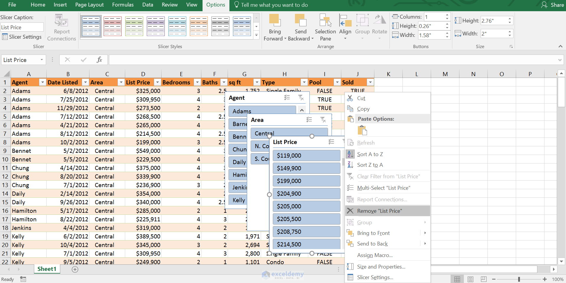 1917×959 slicers filter table excel exceldemycom from www.exceldemy.com
  640×402 excel pivot table slicers filters overhauled pakaccountantscom from pakaccountants.com
  768×558 slicers excel filter data from www.free-power-point-templates.com
  640×296 filter excel pivot tables slicers exceldemy from www.exceldemy.com
 How To Use Pivot Table Slicers To Filter Data In Excel was posted in September 19, 2025 at 5:51 am. If you wanna have it as yours, please click the Pictures and you will go to click right mouse then Save Image As and Click Save and download the How To Use Pivot Table Slicers To Filter Data In Excel Picture.. Don’t forget to share this picture with others via Facebook, Twitter, Pinterest or other social medias! we do hope you'll get inspired by ExcelKayra... Thanks again! If you have any DMCA issues on this post, please contact us!