How To Use The Indirect Function For Dynamic Ranges In Excel
How To Use The Indirect Function For Dynamic Ranges In Excel - There are a lot of affordable templates out there, but it can be easy to feel like a lot of the best cost a amount of money, require best special design template. Making the best template format choice is way to your template success. And if at this time you are looking for information and ideas regarding the How To Use The Indirect Function For Dynamic Ranges In Excel then, you are in the perfect place. Get this How To Use The Indirect Function For Dynamic Ranges In Excel for free here. We hope this post How To Use The Indirect Function For Dynamic Ranges In Excel inspired you and help you what you are looking for.
“`html
Using the INDIRECT Function for Dynamic Ranges in Excel
The INDIRECT function in Excel is a powerful tool that allows you to use text strings to create cell references. This is particularly useful for creating dynamic ranges, which automatically adjust their size as data is added or removed from a spreadsheet. Dynamic ranges can significantly streamline tasks like creating charts, performing calculations on varying datasets, and managing large lists.
Understanding the INDIRECT Function
The basic syntax of the INDIRECT function is:
=INDIRECT(ref_text, [a1])- ref_text: This is the text string that represents the cell reference you want to use. It can be a cell containing the text of a cell reference (e.g., “A1”), a calculated string that constructs a cell reference (e.g., “A”&ROW()), or a named range (e.g., “MyRange”).
- [a1]: This is an optional argument that specifies the referencing style of
ref_text. If set to TRUE (or omitted), INDIRECT interpretsref_textas an A1-style reference (e.g., “A1”, “B10”). If set to FALSE, INDIRECT interpretsref_textas an R1C1-style reference (e.g., “R1C1”, “R10C2”). In most cases, you’ll use the A1 style (TRUE or omitted).
The key is that INDIRECT *evaluates* the text string in ref_text and converts it into an actual cell reference. This indirect approach is what makes dynamic ranges possible.
Creating a Simple Dynamic Range with Named Ranges
One of the easiest ways to create a dynamic range using INDIRECT is in conjunction with named ranges. Let’s say you have a list of data in column A, starting from cell A2, and you want to create a dynamic range that includes all the entries in that list.
- Define a Named Range for the Starting Cell: Select cell A2 (the first cell containing data) and go to the Formulas tab. Click “Define Name”. In the “Name” field, enter a name like “DataStart”. The “Refers to” field should show “=Sheet1!$A$2” (assuming your sheet is named Sheet1). Click OK.
- Determine the Last Cell Dynamically: You need a way to find the last cell containing data in column A. The COUNTA function can help with this. COUNTA counts the number of non-empty cells in a range. Assuming your data is contiguous (no blank cells within the data), the following formula will give you the row number of the last cell:
- Define a Named Range for the Last Row: It’s often helpful to define a name for the row number of the last cell. Create another named range (Formulas tab -> Define Name). Name it something like “LastRow”. In the “Refers to” field, enter the COUNTA formula:
- Use INDIRECT to Create the Dynamic Range: Now, use the INDIRECT function to create the dynamic range. You’ll construct a text string that represents the entire range using the named ranges you’ve defined. For example, let’s say you want to create a named range called “MyDynamicRange”. Go to Formulas tab -> Define Name. In the “Name” field, enter “MyDynamicRange”. In the “Refers to” field, enter the following formula:
"Sheet1!A": This is the starting part of the cell reference string. It specifies column A on Sheet1.&DataStart: This concatenates the string “Sheet1!A” with the value of the “DataStart” named range, which is 2 (the row number of the first data cell). So, the string becomes “Sheet1!A2”.":A": This adds the colon (“:”) to indicate a range, followed by “A” for column A again.&LastRow: This concatenates the string with the value of the “LastRow” named range, which represents the last row number containing data. For example, if the last row with data is 10, this will be 10.INDIRECT(...): The entire string is passed to INDIRECT, which evaluates it as a cell range reference: “Sheet1!A2:A10” (in this example).
=COUNTA(A:A)This counts all non-blank cells in column A.
=COUNTA(Sheet1!A:A)(Adjust “Sheet1” to the name of your actual sheet.)
Click OK.
=INDIRECT("Sheet1!A"&DataStart&":A"&LastRow)(Adjust “Sheet1” to the name of your actual sheet.)
Click OK.
Explanation of the Formula:
Now, whenever you add or remove data from column A, “MyDynamicRange” will automatically adjust to include only the cells containing data. You can use this dynamic range in charts, formulas (SUM, AVERAGE, etc.), or as a data source for other features in Excel.
Using OFFSET and COUNTA within INDIRECT (More Robust)
While the above method works well for contiguous data, it can fail if there are blank cells within your data. A more robust approach uses the OFFSET function in combination with COUNTA within INDIRECT.
The OFFSET function allows you to specify a starting cell and then move a certain number of rows and columns from that cell to define a range. The syntax is:
=OFFSET(reference, rows, cols, [height], [width])- reference: The starting cell for the offset.
- rows: The number of rows to offset from the starting cell (positive to move down, negative to move up).
- cols: The number of columns to offset from the starting cell (positive to move right, negative to move left).
- [height]: The height (number of rows) of the resulting range (optional).
- [width]: The width (number of columns) of the resulting range (optional).
Here’s how to use OFFSET and COUNTA with INDIRECT to create a dynamic range:
- Name the Starting Cell: Name cell A2 (where your data starts) as “DataStart” (same as before).
- Create the Dynamic Range using INDIRECT and OFFSET: Define a new named range (e.g., “MyDynamicRange2”). In the “Refers to” field, enter the following formula:
- A slightly simpler method using OFFSET: You can also construct the same effect using offset by using the following in the name manager instead of the above, more complex example:
=OFFSET(DataStart,0,0,COUNTA(Sheet1!A:A)-ROW(DataStart)+1,1)(Adjust “Sheet1” to the name of your actual sheet.)
Explanation of the Formula:
- ADDRESS(ROW(DataStart),COLUMN(DataStart)): This portion gets the A1 style reference of DataStart. The ROW and COLUMN functions are used to determine the row and column number of the named range “DataStart”. The ADDRESS function turns those row and column numbers into a cell address like “A2”.
- ADDRESS(ROW(DataStart)+COUNTA(Sheet1!A:A)-ROW(DataStart),COLUMN(DataStart)): This calculates the cell reference of the *last* cell in the dynamic range.
ROW(DataStart): Gets the row number of the starting cell (e.g., 2).COUNTA(Sheet1!A:A): Gets the total number of non-blank cells in column A.ROW(DataStart)+COUNTA(Sheet1!A:A)-ROW(DataStart): Calculates the row number of the last cell containing data, considering potential blank cells within the data. If you have 10 non-blank cells, and your data starts in row 2, this calculates row 11.COLUMN(DataStart): Gets the column number of the starting cell (column A, which is 1).
So, this address gets the last populated cell.
- INDIRECT(…): The INDIRECT function takes the concatenated string “Sheet1!A2:A11” (in this example) and converts it into a valid cell range reference.
=INDIRECT("Sheet1!"&ADDRESS(ROW(DataStart),COLUMN(DataStart))&":"&ADDRESS(ROW(DataStart)+COUNTA(Sheet1!A:A)-ROW(DataStart),COLUMN(DataStart)))(Adjust “Sheet1” to the name of your actual sheet.)
Click OK.
Advantages of Using INDIRECT for Dynamic Ranges
- Flexibility: INDIRECT allows you to create ranges based on various criteria, including the contents of other cells, calculations, and named ranges.
- Readability: While the formulas can be complex, using named ranges makes them more readable and easier to understand.
- Dynamic Updates: Dynamic ranges automatically adjust as your data changes, saving you time and effort.
- Integration with other Excel features: Dynamic ranges can be seamlessly integrated with charts, pivot tables, and other Excel features.
Cautions When Using INDIRECT
- Volatility: The INDIRECT function is volatile, meaning it recalculates whenever *any* cell in the workbook changes, even if the referenced cell hasn’t changed. This can slow down large or complex spreadsheets. Use with caution.
- Error Handling: If the
ref_textargument in INDIRECT doesn’t evaluate to a valid cell reference, the function returns a #REF! error. Ensure your formulas are correct. - Complexity: INDIRECT formulas can become complex and difficult to debug, especially when combined with other functions. Document your formulas well.
In conclusion, the INDIRECT function is a valuable tool for creating dynamic ranges in Excel. While it has its limitations, the flexibility and automation it provides can significantly enhance your spreadsheet capabilities. By understanding the syntax, using named ranges, and being mindful of the volatility, you can effectively leverage INDIRECT to manage and analyze your data more efficiently.
“`
 1024×386 indirect function named ranges excelbuddycom from excelbuddy.com
  1301×586 excel indirect function excelfind from excelfind.com
 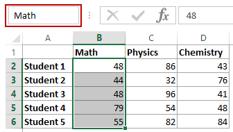 336×190 excel indirect function explained examples video from trumpexcel.com
 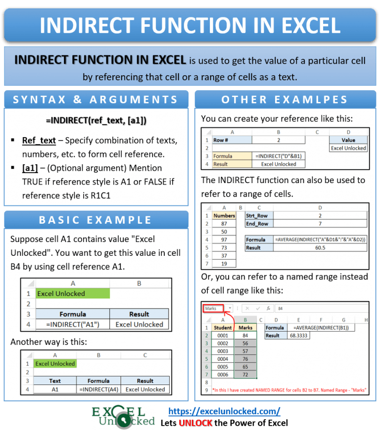 768×881 indirect function excel values reference excel unlocked from excelunlocked.com
  400×215 indirect dynamically reference cell excel aj from www.articlejobber.com
  465×202 excel indirect function excel vba from www.exceldome.com
  767×656 indirect function excel suitable instances from www.exceldemy.com
  800×600 indirect function dailyexcelnet from dailyexcel.net
  514×147 indirect function excel from www.extendoffice.com
  768×247 indirect function excel formulaexamples indirect from www.educba.com
 How To Use The Indirect Function For Dynamic Ranges In Excel was posted in October 8, 2025 at 7:35 pm. If you wanna have it as yours, please click the Pictures and you will go to click right mouse then Save Image As and Click Save and download the How To Use The Indirect Function For Dynamic Ranges In Excel Picture.. Don’t forget to share this picture with others via Facebook, Twitter, Pinterest or other social medias! we do hope you'll get inspired by ExcelKayra... Thanks again! If you have any DMCA issues on this post, please contact us!