Printable Grocery Shopping List Excel With Prices
Printable Grocery Shopping List Excel With Prices - There are a lot of affordable templates out there, but it can be easy to feel like a lot of the best cost a amount of money, require best special design template. Making the best template format choice is way to your template success. And if at this time you are looking for information and ideas regarding the Printable Grocery Shopping List Excel With Prices then, you are in the perfect place. Get this Printable Grocery Shopping List Excel With Prices for free here. We hope this post Printable Grocery Shopping List Excel With Prices inspired you and help you what you are looking for.
Printable Grocery Shopping List Excel with Prices: A Comprehensive Guide
Creating a well-organized grocery shopping list is a cornerstone of efficient and cost-effective meal planning. Utilizing Excel, a readily available and powerful spreadsheet program, you can elevate your shopping list beyond a simple handwritten note. This guide will walk you through building a printable grocery shopping list in Excel that incorporates prices, enabling you to track spending, compare costs, and make informed decisions at the store.
Why Use Excel for Your Grocery List?
While numerous apps and templates cater to grocery shopping, Excel offers unique advantages: * **Customization:** You have complete control over the layout, categories, formulas, and appearance. Tailor the list to your specific needs and preferences. * **Flexibility:** Easily adapt the list to different stores, dietary requirements, or specific recipes. * **Offline Access:** No need for an internet connection. Your list is readily available on your computer or printed. * **Cost Tracking:** Incorporate price information to monitor your spending and identify potential savings. * **Familiarity:** Many users are already comfortable with Excel’s interface, minimizing the learning curve. * **Printable Format:** Creating a printer-friendly layout is straightforward, allowing for a physical copy to take to the store.
Building Your Grocery Shopping List in Excel: Step-by-Step
Follow these steps to create a functional and informative grocery list: **1. Setting Up the Spreadsheet:** * **Open Excel:** Launch Microsoft Excel on your computer. * **Create a New Worksheet:** Start with a blank worksheet. Rename it to “Grocery List” or a similar descriptive title by double-clicking the sheet tab at the bottom of the screen. * **Define Columns:** Determine the essential information you want to track. Consider the following column headers: * **Category:** (e.g., Produce, Dairy, Meat, Pantry, Frozen) – This helps organize your list logically. * **Item:** (e.g., Apples, Milk, Chicken Breast, Pasta, Ice Cream) – The specific item you need to purchase. * **Quantity:** (e.g., 3, 1 gallon, 1 lb, 2 boxes) – The amount you require. * **Unit:** (e.g., each, gallon, lb, box) – Provides clarity on the quantity. (Optional, but recommended for consistency). * **Price per Unit:** (e.g., $1.50, $3.00, $5.99, $2.50) – The cost of one unit of the item. * **Total Price:** (Calculated automatically – see formula below). * **Store:** (e.g., Kroger, Walmart, Trader Joe’s) – Helpful if you shop at multiple stores and prices vary. (Optional). * **Aisle:** (e.g., 1, 5, 10) – If your store is well-organized, this can save time navigating the aisles. (Optional). * **Checked:** (Checkbox or simple “x”) – To mark items as you put them in your cart. * **Adjust Column Widths:** Double-click the line separating column headers to automatically adjust the width to fit the content. You can also manually drag the column dividers. * **Format Headers:** Make the headers stand out by formatting them. Select the header row, and use the formatting tools (font, size, bold, colors) to enhance readability. * **Freeze Top Row:** Select the row *below* the header row (usually row 2). Go to the “View” tab and click “Freeze Panes” then “Freeze Top Row.” This keeps the headers visible as you scroll down the list. **2. Entering Data:** * **Populate the List:** Start filling in your grocery needs, category by category. Be as specific as possible with item names to avoid confusion. * **Quantity and Unit Consistency:** Use consistent units for similar items (e.g., always use “lb” for meat). * **Price Tracking:** Enter the price per unit for each item. If you’re unsure, estimate or look up online prices for your local stores. This step is crucial for cost tracking. You can also create a separate “Price List” sheet (explained later) to pull prices from. **3. Calculating Total Price:** * **The Formula:** In the “Total Price” column, enter the following formula (assuming your “Quantity” is in column C and “Price per Unit” is in column E): `=C2*E2` (Adjust the row number ‘2’ to match the row where you are entering data). * **Autofill:** Click the small square at the bottom right corner of the cell containing the formula and drag it down to apply the formula to all rows with item entries. Excel will automatically adjust the row numbers in the formula for each row. * **Format as Currency:** Select the “Total Price” column (and the “Price per Unit” column), and format it as currency. Go to the “Home” tab, and in the “Number” group, select “Currency” or “Accounting.” Choose your preferred currency symbol (e.g., $). **4. Adding a Total Spending Summary:** * **Create a Summary Section:** At the bottom of your list (or in a designated area), create a section to display your total spending. * **Add a Label:** In a cell, type “Total Estimated Spending:”. * **The SUM Formula:** In the cell next to the label, enter the following formula to sum the “Total Price” column (assuming your “Total Price” column is column F and your data starts in row 2 and ends in row 20. Adjust the range to match your actual data): `=SUM(F2:F20)` * **Format as Currency:** Format the cell containing the sum as currency, just like the “Total Price” column. **5. Enhancing Organization and Visual Appeal:** * **Sorting:** Sort your list by category, aisle, or any other column to make it easier to navigate the store. Select the entire data range (including headers), go to the “Data” tab, and click “Sort.” Choose the column you want to sort by. * **Filtering:** Filter your list to show only specific categories or items from a particular store. Select the entire data range, go to the “Data” tab, and click “Filter.” Drop-down arrows will appear in the header row, allowing you to filter the data. * **Conditional Formatting:** Use conditional formatting to highlight items based on price, category, or any other criteria. Select the data range, go to the “Home” tab, and click “Conditional Formatting.” Explore the different formatting options. * **Color Coding:** Use background colors or text colors to differentiate categories or highlight important items. * **Borders:** Add borders to your list to visually separate sections and improve readability. Select the data range, go to the “Home” tab, and click the “Borders” icon in the “Font” group. * **Checkboxes:** Implement checkboxes for easy tracking. Select the cells in the “Checked” column. Go to the “Developer” tab (if you don’t see it, go to File -> Options -> Customize Ribbon and check the “Developer” box), click “Insert” and choose the checkbox form control. Link the checkbox to a cell to track its state. You can then use conditional formatting to strikethrough completed items. **6. Creating a Printable Version:** * **Page Layout View:** Go to the “View” tab and click “Page Layout.” This will show you how your list will appear when printed. * **Adjust Margins and Orientation:** Go to the “Page Layout” tab. Adjust the margins, orientation (portrait or landscape), and paper size to fit your list onto the page(s) effectively. * **Print Area:** Define the print area to include only the relevant data. Select the data range you want to print, go to the “Page Layout” tab, click “Print Area,” and choose “Set Print Area.” * **Print Titles:** Ensure that the header row appears on every printed page. Go to the “Page Layout” tab, click “Print Titles,” and specify the rows to repeat at the top (usually row 1). * **Scale to Fit:** If your list is too wide to fit on a single page, use the scaling options in the “Page Layout” tab to shrink the content to fit. Be mindful of readability when scaling. **7. Advanced Features:** * **Price List Sheet:** Create a separate sheet (e.g., “Price List”) to store a master list of items and their prices at different stores. Use VLOOKUP or INDEX/MATCH formulas to automatically pull prices from the “Price List” sheet into your grocery list based on the item name and store selection. This will save you time and ensure price consistency. * **Macros:** For repetitive tasks, consider using macros to automate them. For example, you could create a macro to clear the “Checked” column and reset the list for the next shopping trip. * **Data Validation:** Use data validation to restrict the values that can be entered in certain cells, such as the “Category” column, to ensure consistency and prevent errors. * **Pivot Tables:** If you track your spending over time, use pivot tables to analyze your grocery expenses by category, store, or date. **Example Formulas and Tips:** * **VLOOKUP (for Price Lookup):** Assuming your “Price List” sheet has columns “Item” (A), “Price” (B), and your grocery list has “Item” in column B and “Store” in column D, the formula in the “Price per Unit” column (E) would be: `=VLOOKUP(B2, ‘Price List’!A:B, 2, FALSE)` (This looks for the Item in B2 within the Price List, and returns the corresponding price). You might need to combine this with an IF statement to select the correct price based on the “Store.” * **IF Statement (for Store-Specific Pricing with VLOOKUP):** `=IF(D2=”Kroger”, VLOOKUP(B2, ‘Price List’!A:C, 2, FALSE), IF(D2=”Walmart”, VLOOKUP(B2, ‘Price List’!A:C, 3, FALSE), “Price Not Found”))` (This checks the Store, then uses VLOOKUP to find the price in the corresponding column of the Price List) * **INDEX/MATCH (Alternative to VLOOKUP):** INDEX/MATCH is more flexible than VLOOKUP. It doesn’t require the lookup value to be in the first column of the lookup table. `=INDEX(‘Price List’!B:B, MATCH(B2, ‘Price List’!A:A, 0))` (This finds the Item in column A of the Price List and returns the price from column B).
Conclusion
By creating a printable grocery shopping list in Excel with prices, you gain greater control over your spending and streamline your shopping trips. The ability to track prices, calculate totals, and organize your list efficiently will save you time and money in the long run. Don’t be afraid to experiment with different features and formulas to customize your list to perfectly suit your needs. Remember to update your price information regularly to maintain accuracy. Happy shopping!
 790×624 grocery shopping list templates google sheets microsoft from slidesdocs.com
  1400×758 grocery spreadsheet grocery shopping list excel template from db-excel.com
  1203×873 grocery shopping list excel template printable grocery list editable from www.pinterest.com
  3000×1688 grocery shopping list excel from fity.club
 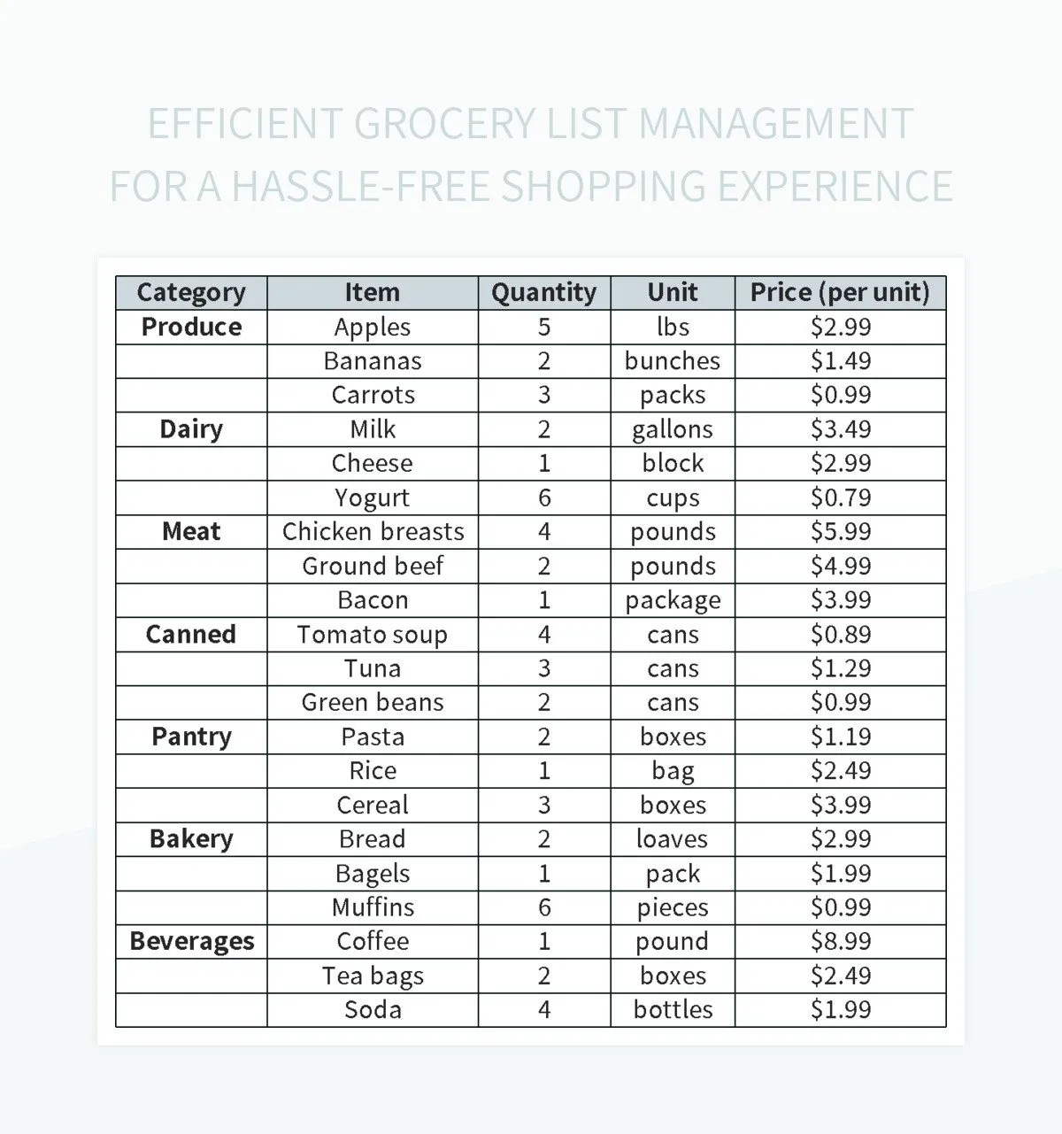 1200×1281 grocery list templates google sheets microsoft excel from slidesdocs.com
  1920×1039 grocery list spreadsheet household shopping list excel from db-excel.com
  1218×1545 printable grocery list prices from mungfali.com
  550×534 grocery list spreadsheet printable editable food shopping planner from www.buyexceltemplates.com
  601×778 grocery spreadsheet template regard grocery shopping list from db-excel.com
  996×1200 editable excel grocery list templatesfree from www.ziplist.com
  1361×1761 grocery list template printable from www.101planners.com
  1237×1600 grocery shopping list excel cynthia jasmin blog from storage.googleapis.com
  3000×2318 grocery shopping list excel template unit price cost editable from www.etsy.com
  950×699 grocery list template excel downloadxlsx from techguruplus.com
  1080×783 top grocery list excel template ultimate guide from softwareaccountant.com
  723×558 family grocery list excel format templates excel templates from www.dotxls.org
  828×657 excel spreadsheet template list template templates golden delicious from www.pinterest.co.kr
  600×845 printable grocery list shopping list templates excel from www.spreadsheet123.com
  2426×3026 grocery list coupons spreadsheet db excelcom from db-excel.com
  703×552 editable grocery list template excel from upload.independent.com
  600×816 grocery list excel template from data1.skinnyms.com
  540×405 grocery shopping list template google sheets excel spreadsheet excel from www.pinterest.ca
  540×405 computer screen checklist words excel from www.pinterest.com
  1080×1080 grocery list template excel printable organize etsy from www.etsy.com
  600×506 grocery list template excel price list template from www.heritagechristiancollege.com
  860×539 excel grocery list template from templates.rjuuc.edu.np
  1926×1442 excel simple grocery listxlsx wps templates from template.wps.com
  1760×1140 grocery list template excel google sheets templatenet from www.template.net
  700×724 grocery list template shopping lists excel word from www.docformats.com
  431×560 excel shopping list template from animalia-life.club
 Printable Grocery Shopping List Excel With Prices was posted in October 5, 2025 at 8:33 am. If you wanna have it as yours, please click the Pictures and you will go to click right mouse then Save Image As and Click Save and download the Printable Grocery Shopping List Excel With Prices Picture.. Don’t forget to share this picture with others via Facebook, Twitter, Pinterest or other social medias! we do hope you'll get inspired by ExcelKayra... Thanks again! If you have any DMCA issues on this post, please contact us!