Vlookup Approximate Match Formula Tutorial In Excel
Vlookup Approximate Match Formula Tutorial In Excel - There are a lot of affordable templates out there, but it can be easy to feel like a lot of the best cost a amount of money, require best special design template. Making the best template format choice is way to your template success. And if at this time you are looking for information and ideas regarding the Vlookup Approximate Match Formula Tutorial In Excel then, you are in the perfect place. Get this Vlookup Approximate Match Formula Tutorial In Excel for free here. We hope this post Vlookup Approximate Match Formula Tutorial In Excel inspired you and help you what you are looking for.
“`html
VLOOKUP Approximate Match: A Comprehensive Guide
The VLOOKUP function in Excel is a powerful tool for retrieving data from a table based on a lookup value. While the exact match VLOOKUP is commonly used, the approximate match option (set by specifying TRUE or omitting the fourth argument) unlocks a new dimension of possibilities. This guide will delve into the intricacies of the approximate match VLOOKUP, explaining how it works, when to use it, and potential pitfalls to avoid.
Understanding the Approximate Match
Unlike the exact match, which returns an error if the lookup value isn’t found exactly, the approximate match VLOOKUP seeks the nearest match. Specifically, it finds the largest value in the first column of the lookup table that is less than or equal to the lookup value.
Important Prerequisites:
- Sorted Lookup Column: The most crucial requirement for the approximate match VLOOKUP is that the first column of your lookup table (the column containing the values you’re searching against) must be sorted in ascending order (smallest to largest). Failure to sort the data correctly will lead to unpredictable and often incorrect results.
- Understanding the Logic: Remember, VLOOKUP will stop when it encounters the first value in the lookup column that is *greater* than the lookup value. It will then return the value from the row *before* that one, assuming that’s the closest match that’s still less than or equal to the lookup value.
The VLOOKUP Formula Structure (Approximate Match)
The general structure of the VLOOKUP formula with approximate match is:
=VLOOKUP(lookup_value, table_array, col_index_num, [range_lookup])
Where:
lookup_value: The value you’re searching for in the first column of the table.table_array: The range of cells containing your lookup table (including the lookup column and the column containing the value you want to return).col_index_num: The column number within thetable_arrayfrom which the matching value should be returned. The leftmost column is column 1.[range_lookup]: An optional argument. If omitted or set toTRUE, VLOOKUP performs an approximate match. Setting it toFALSEenforces an exact match.
When to Use Approximate Match VLOOKUP
Approximate match VLOOKUP excels in scenarios where you need to categorize values or apply a tiered system based on ranges:
- Grading Systems: Assigning letter grades (A, B, C, etc.) based on numerical scores. You would create a table with minimum scores for each grade, and VLOOKUP would find the appropriate grade based on a student’s score.
- Tax Brackets: Calculating income tax based on income ranges.
- Commission Rates: Determining commission rates based on sales volume tiers.
- Shipping Costs: Calculating shipping costs based on weight or distance ranges.
- Age Groups: Categorizing individuals into age groups like child, teenager, adult, senior.
Examples
Example 1: Grading System
Suppose you have the following grading scale:
| Score | Grade |
|---|---|
| 0 | F |
| 60 | D |
| 70 | C |
| 80 | B |
| 90 | A |
This table is in the range A1:B5. Now, let’s say a student has a score of 75 in cell D2. The following formula would return “C”:
=VLOOKUP(D2, A1:B5, 2, TRUE)
Explanation:
D2(75) is thelookup_value.A1:B5is thetable_array.2indicates that the value from the second column (Grade) should be returned.TRUEspecifies an approximate match.
VLOOKUP searches the first column (Score). It finds 0, 60, 70, and then encounters 80. Since 80 is greater than 75, it returns the value from the row *before* that one (70), and then returns the corresponding grade from column 2 (C).
Example 2: Commission Rates
Let’s say you have a commission structure like this:
| Sales Volume | Commission Rate |
|---|---|
| 0 | 0% |
| 10000 | 2% |
| 25000 | 5% |
| 50000 | 7.5% |
| 100000 | 10% |
This table is in the range E1:F5. A salesperson has sales of $35,000 in cell G2. To calculate the commission rate, you would use:
=VLOOKUP(G2, E1:F5, 2, TRUE)
This formula would return 5%.
Common Pitfalls and Troubleshooting
- Unsorted Data: This is the biggest culprit! Always double-check that the first column of your lookup table is sorted in ascending order. Excel’s sorting feature can easily handle this (Data -> Sort).
- Incorrect Column Index: Ensure that
col_index_numaccurately reflects the column containing the value you want to return. A common mistake is off-by-one errors. - Data Type Mismatches: Ensure the data type of your
lookup_valueis compatible with the data type in the first column of yourtable_array. For example, if you’re looking up a number, make sure the first column contains numbers and not text. - Values Below the Lowest Value in the Lookup Table: If the
lookup_valueis less than the smallest value in the first column of thetable_array, VLOOKUP will return#N/A. This is because it can’t find a value that’s less than or equal to thelookup_value. Consider adding a row with a minimum value (e.g., 0 in the grading example) to avoid this. - Unexpected Results: If you’re getting results that don’t seem right, carefully examine your data and the logic of your formula. Step through the formula using Excel’s “Evaluate Formula” tool (Formulas -> Evaluate Formula) to understand how VLOOKUP is processing the data.
Alternatives to Approximate Match VLOOKUP
While VLOOKUP with approximate match is useful, other functions can sometimes provide more flexibility or clarity:
- INDEX and MATCH: This combination is often preferred over VLOOKUP because it’s less prone to errors related to column order. You can use MATCH to find the row number that corresponds to your approximate match, and then INDEX to return the value from the desired column.
- XLOOKUP: A newer function available in Excel 365 and later versions, XLOOKUP offers several advantages over VLOOKUP, including built-in approximate matching options and the ability to search both horizontally and vertically. It handles errors more gracefully and doesn’t require the lookup column to be the leftmost column.
- IF Statements: For simpler scenarios with a small number of categories, nested IF statements might be easier to understand and maintain. However, they become unwieldy for complex situations.
Conclusion
The approximate match VLOOKUP is a valuable tool for a wide range of data analysis tasks. By understanding its logic, adhering to the requirement of sorted data, and carefully considering potential pitfalls, you can leverage its power to efficiently categorize data and automate calculations based on value ranges. Remember to explore alternative functions like INDEX/MATCH and XLOOKUP to determine the best approach for your specific needs.
“`
 768×367 vlookup approximate match myexcelonline from www.myexcelonline.com
  1280×720 excel tutorial troubleshoot vlookup approximate match from exceljet.net
 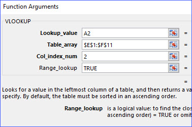 378×251 vlookup approximate match excelnotes from excelnotes.com
  474×234 vlookup exact approximate match excel from www.extendoffice.com
  1280×720 vlookup approximate match microsoft excel basic advanced from www.goskills.com
  405×297 excel vlookup tutorial beginners formula examples from ablebits.com
  1280×600 exact approximate matching vlookup excel from ms-office.wonderhowto.com
 Vlookup Approximate Match Formula Tutorial In Excel was posted in November 27, 2025 at 7:53 pm. If you wanna have it as yours, please click the Pictures and you will go to click right mouse then Save Image As and Click Save and download the Vlookup Approximate Match Formula Tutorial In Excel Picture.. Don’t forget to share this picture with others via Facebook, Twitter, Pinterest or other social medias! we do hope you'll get inspired by ExcelKayra... Thanks again! If you have any DMCA issues on this post, please contact us!