Vlookup Approximate Match Tutorial In Excel
Vlookup Approximate Match Tutorial In Excel - There are a lot of affordable templates out there, but it can be easy to feel like a lot of the best cost a amount of money, require best special design template. Making the best template format choice is way to your template success. And if at this time you are looking for information and ideas regarding the Vlookup Approximate Match Tutorial In Excel then, you are in the perfect place. Get this Vlookup Approximate Match Tutorial In Excel for free here. We hope this post Vlookup Approximate Match Tutorial In Excel inspired you and help you what you are looking for.
“`html
VLOOKUP Approximate Match: A Comprehensive Guide
VLOOKUP is a powerful Excel function for finding data in a table. While many users are familiar with the exact match feature, VLOOKUP’s approximate match functionality offers a versatile solution for situations where you need to find the closest value within a specified range. This tutorial will guide you through the intricacies of VLOOKUP approximate match, explaining its mechanics, benefits, and providing practical examples to enhance your understanding.
Understanding the VLOOKUP Function
Before delving into approximate match, let’s review the fundamental structure of the VLOOKUP function:
=VLOOKUP(lookup_value, table_array, col_index_num, [range_lookup])
- lookup_value: The value you want to search for in the first column of the table.
- table_array: The range of cells containing the table where the data resides. The lookup value must be in the first column of this range.
- col_index_num: The column number within the `table_array` from which to retrieve the matching value. Counting starts from the leftmost column of the `table_array`.
- range_lookup: This is where the magic of exact versus approximate match happens.
TRUE(or omitted): Performs an approximate match. The function assumes the first column of `table_array` is sorted in ascending order. If an exact match is not found, it will return the next largest value that is less than the `lookup_value`.FALSE: Performs an exact match. The function will only return a value if an exact match to the `lookup_value` is found in the first column of the `table_array`. If no exact match is found, it returns an error (#N/A).
The Power of Approximate Match
Approximate match shines when you need to categorize data based on ranges. Imagine scenarios like:
- Grading Systems: Assigning letter grades based on numerical scores (e.g., 90-100 = A, 80-89 = B).
- Commission Tiers: Calculating sales commissions based on sales volume ranges.
- Tax Brackets: Determining the applicable tax rate based on income brackets.
- Shipping Costs: Calculating shipping costs based on weight ranges.
In these situations, you don’t need an exact match for a value. Instead, you want to find the corresponding category or value based on where your `lookup_value` falls within the defined ranges.
How Approximate Match Works
When `range_lookup` is set to `TRUE` (or omitted), VLOOKUP operates differently:
- Assumed Sorted Order: It requires the first column of your `table_array` (the lookup column) to be sorted in ascending order. If the data is not sorted correctly, the results will be unpredictable and likely incorrect.
- Searching for a Match: VLOOKUP starts searching down the first column for the `lookup_value`.
- Exact Match Found: If an exact match is found, VLOOKUP returns the corresponding value from the column specified by `col_index_num`.
- No Exact Match Found: If VLOOKUP doesn’t find an exact match, it continues searching until it finds a value that is greater than the `lookup_value`.
- Returning the Previous Value: VLOOKUP then returns the value from the *previous* row in the column specified by `col_index_num`. This is the key to approximate matching: it returns the largest value that is less than or equal to the `lookup_value`.
Example: Grading System
Let’s create a grading system where scores are assigned letter grades:
Table (A1:B5):
| Score | Grade |
|---|---|
| 0 | F |
| 60 | D |
| 70 | C |
| 80 | B |
| 90 | A |
Now, let’s say we have a score in cell D1, and we want to determine the corresponding grade in cell E1. We can use the following VLOOKUP formula:
=VLOOKUP(D1, A1:B5, 2, TRUE)
Here’s how it works for different scores in D1:
- D1 = 85: VLOOKUP searches column A. It doesn’t find 85. It finds that 90 is the first value greater than 85. It then goes back to the previous row (80) and returns the corresponding value from column 2, which is “B”.
- D1 = 70: VLOOKUP finds an exact match of 70 in column A. It returns the corresponding value from column 2, which is “C”.
- D1 = 50: VLOOKUP searches column A. It finds that 60 is the first value greater than 50. It goes back to the previous row (0) and returns the corresponding value from column 2, which is “F”.
- D1 = 95: VLOOKUP searches column A. It doesn’t find 95. Because 90 is the *last* value and no value is greater than 95, the function returns the grade associated with 90, which is “A”.
Important Considerations
- Sorted Data is Crucial: The absolute most important thing to remember is that the first column of your `table_array` *must* be sorted in ascending order for approximate match to work correctly. Excel will not warn you if the data is not sorted; it will simply return incorrect results.
- Lowest Value: Your table should typically include the lowest possible value in the range. In the grading example, we included 0 to ensure that any score below 60 is correctly assigned an “F”.
- Boundaries: Pay careful attention to the boundaries between ranges. In our grading example, a score of 80 will result in a “B,” while a score of 79.99 (or any value less than 80) will result in a “C.”
- Error Handling: If your `lookup_value` is less than the smallest value in the first column of your `table_array`, VLOOKUP will still return a value. Be sure that this is intended behavior. Consider using an `IF` statement or `IFERROR` function to handle cases where the `lookup_value` is outside of the expected range.
- Alternative Approaches: While VLOOKUP with approximate match is effective, other functions like `IFS` or `LOOKUP` might provide more readable or flexible solutions in certain scenarios. Consider these alternatives based on the complexity of your logic.
Example: Commission Tiers
Let’s illustrate with another example, commission tiers based on sales volume:
Table (A1:B4):
| Sales Volume | Commission Rate |
|---|---|
| 0 | 0% |
| 10000 | 5% |
| 25000 | 7.5% |
| 50000 | 10% |
If cell D1 contains the sales volume, the following formula in E1 will calculate the commission rate:
=VLOOKUP(D1, A1:B4, 2, TRUE)
For example:
- D1 = 30000: VLOOKUP returns 7.5% because 30000 falls between 25000 and 50000. The largest value less than or equal to 30000 is 25000, so the associated commission rate is returned.
- D1 = 8000: VLOOKUP returns 0% because 8000 is less than 10000. The largest value less than or equal to 8000 is 0, so the associated commission rate is returned.
- D1 = 50000: VLOOKUP returns 10% because it finds an exact match for 50000.
Troubleshooting
If you’re experiencing issues with VLOOKUP approximate match, consider the following:
- Data Sorting: Double-check that the first column of your `table_array` is sorted in ascending order. This is the most common cause of errors.
- Data Types: Ensure that the `lookup_value` and the values in the first column of your `table_array` have compatible data types (e.g., both are numbers or both are text).
- Table Range: Verify that the `table_array` covers the correct range of cells.
- Column Index: Ensure that `col_index_num` is a valid column number within the `table_array`.
- Unexpected Results: If the returned value seems incorrect, carefully review your data and the logic of the VLOOKUP function. Use the Evaluate Formula feature in Excel (Formulas tab -> Formula Auditing -> Evaluate Formula) to step through the calculation and identify the source of the error.
Conclusion
VLOOKUP with approximate match is a valuable tool for categorizing data and finding values within ranges. By understanding its mechanics and adhering to the crucial requirement of sorted data, you can effectively leverage its power in your Excel workflows. Remember to carefully consider the boundary conditions and potential edge cases to ensure accurate and reliable results.
“`
 1024×409 vlookup approximate match myexcelonline from www.myexcelonline.com
  1280×720 excel tutorial troubleshoot vlookup approximate match from exceljet.net
 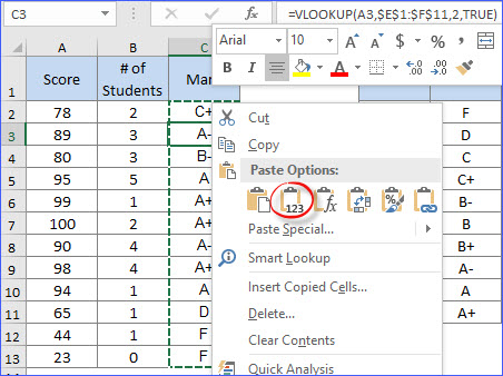 452×338 vlookup approximate match excelnotes from excelnotes.com
  1187×477 vlookup exact approximate match excel from www.extendoffice.com
  481×418 perform approximate match fuzzy lookups excel excel university from www.excel-university.com
  1280×720 vlookup approximate match microsoft excel basic advanced from www.goskills.com
  405×297 excel vlookup tutorial beginners formula examples from ablebits.com
  1280×600 exact approximate matching vlookup excel from ms-office.wonderhowto.com
 Vlookup Approximate Match Tutorial In Excel was posted in January 31, 2026 at 4:48 pm. If you wanna have it as yours, please click the Pictures and you will go to click right mouse then Save Image As and Click Save and download the Vlookup Approximate Match Tutorial In Excel Picture.. Don’t forget to share this picture with others via Facebook, Twitter, Pinterest or other social medias! we do hope you'll get inspired by ExcelKayra... Thanks again! If you have any DMCA issues on this post, please contact us!