How To Use Index And Match Instead Of Vlookup In Excel
How To Use Index And Match Instead Of Vlookup In Excel - There are a lot of affordable templates out there, but it can be easy to feel like a lot of the best cost a amount of money, require best special design template. Making the best template format choice is way to your template success. And if at this time you are looking for information and ideas regarding the How To Use Index And Match Instead Of Vlookup In Excel then, you are in the perfect place. Get this How To Use Index And Match Instead Of Vlookup In Excel for free here. We hope this post How To Use Index And Match Instead Of Vlookup In Excel inspired you and help you what you are looking for.
Unleashing the Power of INDEX and MATCH: A VLOOKUP Alternative in Excel
VLOOKUP has long been a staple in the Excel toolkit, a go-to function for retrieving data from tables based on a lookup value. However, while VLOOKUP is user-friendly and widely understood, it has limitations that can be overcome by using the more flexible and robust combination of INDEX and MATCH. This guide will demonstrate why INDEX and MATCH is often a superior alternative to VLOOKUP and explain how to effectively utilize them.
Why INDEX and MATCH Over VLOOKUP?
Several key advantages make INDEX and MATCH a better choice in many situations: * **Flexibility in Column Order:** VLOOKUP relies on the lookup value being in the leftmost column of the table array. If the column containing the lookup value is not the first, or if you need to insert or delete columns before the lookup column, VLOOKUP will break. INDEX and MATCH are not restricted by column order. They can retrieve data from any column in the table array regardless of its position relative to the lookup column. * **Improved Robustness:** Changes to the table structure can easily disrupt VLOOKUP formulas. Inserting or deleting columns to the left of the lookup column will cause the formula to return incorrect results because the column index number will be off. INDEX and MATCH formulas are more resilient to such changes as they reference columns and rows independently using MATCH to find the row number and INDEX to return the value from that row and specified column. * **Performance with Large Datasets:** While the performance difference may not be noticeable with smaller datasets, INDEX and MATCH generally perform better than VLOOKUP with large tables, especially when searching for exact matches. * **Right-to-Left Lookups:** VLOOKUP cannot perform lookups from right to left, meaning the lookup column must always be to the left of the column containing the value you want to return. INDEX and MATCH easily handle right-to-left lookups, providing a significant advantage.
Understanding the INDEX and MATCH Functions
Before we dive into using them together, let’s understand the individual functions: * **INDEX Function:** The INDEX function returns the value of a cell within a specified range, based on the row and column number. Its basic syntax is: `INDEX(array, row_num, [column_num])` * `array`: The range of cells to search within. * `row_num`: The row number within the array from which to return a value. * `column_num` (optional): The column number within the array from which to return a value. If omitted, it defaults to 1, assuming you are working with a single-column array. * **MATCH Function:** The MATCH function searches for a specified value within a range of cells and returns the *relative position* of that value. Its basic syntax is: `MATCH(lookup_value, lookup_array, [match_type])` * `lookup_value`: The value you want to find. * `lookup_array`: The range of cells to search within. * `match_type` (optional): Specifies how MATCH should match the `lookup_value`. * `0` (Exact match): This is the most common and recommended setting. It finds the first value that is exactly equal to `lookup_value`. * `1` (Less than): Finds the largest value that is less than or equal to `lookup_value`. The `lookup_array` must be sorted in ascending order. * `-1` (Greater than): Finds the smallest value that is greater than or equal to `lookup_value`. The `lookup_array` must be sorted in descending order.
Putting INDEX and MATCH Together: The Magic Formula
The power of INDEX and MATCH comes from combining them. MATCH finds the row number containing the lookup value, and INDEX then uses that row number to retrieve the corresponding value from a different column in the same row. The general formula is: `INDEX(return_column, MATCH(lookup_value, lookup_column, 0))` Let’s break this down: * `return_column`: This is the range of cells containing the value you want to retrieve (e.g., `C2:C10`). * `MATCH(lookup_value, lookup_column, 0)`: This part of the formula uses the MATCH function to find the row number where the `lookup_value` is found in the `lookup_column` (e.g., `B2:B10`). The `0` ensures an exact match. **Example:** Imagine you have a table with employee IDs in column B (B2:B10), names in column A (A2:A10), and salaries in column C (C2:C10). You want to find the salary of the employee with ID “12345”. 1. `lookup_value`: “12345” 2. `lookup_column`: `B2:B10` (the column containing employee IDs) 3. `return_column`: `C2:C10` (the column containing salaries) The formula would be: `=INDEX(C2:C10, MATCH(“12345”, B2:B10, 0))` This formula will: 1. `MATCH(“12345”, B2:B10, 0)`: Search for “12345” in the range B2:B10 and return its row number (e.g., if “12345” is found in cell B5, MATCH will return 4). 2. `INDEX(C2:C10, 4)`: Use the row number (4) returned by MATCH to retrieve the value from the range C2:C10 at the 4th row (which is C5). This returns the salary of the employee with ID “12345”.
Handling Errors
Like VLOOKUP, INDEX and MATCH will return an error (`#N/A`) if the `lookup_value` is not found in the `lookup_column`. You can use the `IFERROR` function to handle these errors gracefully: `=IFERROR(INDEX(C2:C10, MATCH(“12345”, B2:B10, 0)), “Employee ID not found”)` This will display “Employee ID not found” if the employee ID is not in the table.
Two-Dimensional Lookups with INDEX and MATCH
INDEX and MATCH can also be used for two-dimensional lookups, finding values based on both row and column criteria. This is a significant advantage over VLOOKUP, which is limited to one-dimensional lookups. For example, if you have a table of sales data with products in rows and months in columns, you can use INDEX and MATCH to find the sales figure for a specific product in a specific month. The formula would look something like this: `=INDEX(data_range, MATCH(row_lookup_value, row_lookup_range, 0), MATCH(column_lookup_value, column_lookup_range, 0))` * `data_range`: The entire table containing the sales figures. * `row_lookup_value`: The product name you’re searching for. * `row_lookup_range`: The column containing the product names. * `column_lookup_value`: The month you’re searching for. * `column_lookup_range`: The row containing the month names.
Conclusion
INDEX and MATCH offer a more powerful and flexible alternative to VLOOKUP in Excel. By understanding how these functions work individually and how to combine them effectively, you can overcome the limitations of VLOOKUP and create more robust, adaptable, and efficient formulas. Whether you’re dealing with complex data structures, large datasets, or simply want to avoid the pitfalls of VLOOKUP’s column-order dependency, INDEX and MATCH are essential tools for any serious Excel user. Mastering them will significantly enhance your ability to analyze and manipulate data within spreadsheets.
 589×316 index match vlookup kingexcelinfo from www.kingexcel.info
  830×427 index match excel formula guide from excelchamps.com
  324×201 index match vlookup learn microsoft excel from fiveminutelessons.com
 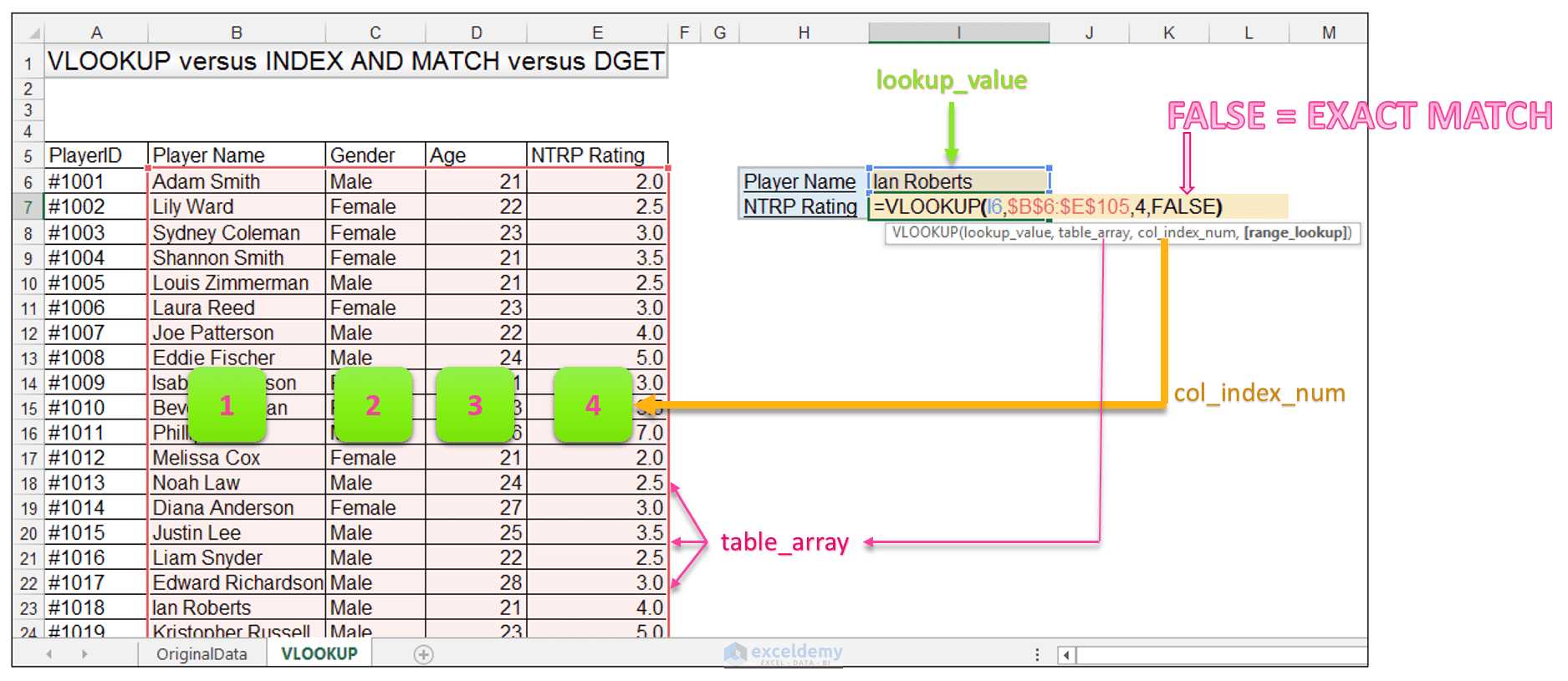 1875×815 index match vlookup dget excel functions comparison from www.exceldemy.com
  450×450 index match great alternative vlookup excel from professor-excel.com
  300×161 index match vlookup excel campus from www.excelcampus.com
  722×499 index match vlookup hlookup excel from quadexcel.com
  674×350 vlookup index match examples excel from www.vertex42.com
 How To Use Index And Match Instead Of Vlookup In Excel was posted in January 16, 2026 at 7:15 pm. If you wanna have it as yours, please click the Pictures and you will go to click right mouse then Save Image As and Click Save and download the How To Use Index And Match Instead Of Vlookup In Excel Picture.. Don’t forget to share this picture with others via Facebook, Twitter, Pinterest or other social medias! we do hope you'll get inspired by ExcelKayra... Thanks again! If you have any DMCA issues on this post, please contact us!