How To Do Conditional Formatting Based On Another Cell In Excel
How To Do Conditional Formatting Based On Another Cell In Excel - There are a lot of affordable templates out there, but it can be easy to feel like a lot of the best cost a amount of money, require best special design template. Making the best template format choice is way to your template success. And if at this time you are looking for information and ideas regarding the How To Do Conditional Formatting Based On Another Cell In Excel then, you are in the perfect place. Get this How To Do Conditional Formatting Based On Another Cell In Excel for free here. We hope this post How To Do Conditional Formatting Based On Another Cell In Excel inspired you and help you what you are looking for.
Conditional Formatting Based on Another Cell in Excel
Conditional formatting is a powerful tool in Excel that allows you to automatically apply formatting (like colors, fonts, and borders) to cells based on specific criteria. While often used to highlight cells based on their own values, conditional formatting becomes even more versatile when you base it on the value of another cell. This technique lets you create dynamic and insightful spreadsheets that visually represent relationships and dependencies between different data points.
Why Use Conditional Formatting Based on Another Cell?
There are numerous scenarios where formatting one cell based on the value of another is incredibly useful:
- Tracking Progress: Highlight project tasks (column A) based on their completion status in another column (column B).
- Inventory Management: Identify products (column A) that are running low based on their stock levels in another column (column B).
- Sales Performance: Highlight sales figures (column A) if they exceed a target set in a specific cell (e.g., cell B1).
- Data Validation: Highlight data entry fields (column A) if their values don’t match requirements defined in another column (column B).
- Creating Visual Alerts: Draw attention to specific rows or columns based on conditions met elsewhere in the spreadsheet.
Methods for Conditional Formatting Based on Another Cell
Excel provides several ways to achieve this type of conditional formatting:
- Using a Formula: This is the most flexible and commonly used method. You create a formula that references the other cell and evaluates to TRUE or FALSE. If the formula is TRUE for a given cell, the specified formatting is applied.
- Using “Use a Formula to Determine Which Cells to Format”: This option, found within the conditional formatting rules manager, lets you define complex conditions based on cell references.
Step-by-Step Guide: Using a Formula for Conditional Formatting
Let’s illustrate this with a practical example. Suppose you have a list of tasks in column A (A1:A10) and their corresponding status (e.g., “Complete,” “In Progress,” “Not Started”) in column B (B1:B10). You want to highlight the entire row of tasks that are marked as “Complete” in column B.
- Select the Range to Format: Select the cells you want to apply the conditional formatting to. In this case, select A1:A10 (the task descriptions). You can extend the selection to include other columns if you want to highlight the entire row, such as A1:C10 (if column C contains further task-related information).
- Open the Conditional Formatting Menu: Go to the “Home” tab on the Excel ribbon and click on “Conditional Formatting” in the “Styles” group.
- Create a New Rule: Choose “New Rule…” from the dropdown menu.
- Select Rule Type: In the “New Formatting Rule” dialog box, select “Use a formula to determine which cells to format.”
- Enter the Formula: In the “Format values where this formula is true” box, enter the following formula:
=$B1="Complete"Important Explanation:
- `=$B1`: This is the crucial part. It refers to the first cell in the column containing the status (B1). The `$` symbol before the “B” makes the column reference absolute. This means that when the formula is applied to other cells in your selected range (A2, A3, etc.), the column being checked will *always* be column B. However, the row number *will* change relative to the row you are formatting. This allows you to check the status in B2 when formatting A2, the status in B3 when formatting A3, and so on.
- `=”Complete”`: This part of the formula specifies the condition you are checking for. It compares the value in cell B1 (or B2, B3, etc. as the formatting is applied) to the text string “Complete”. The text must be enclosed in double quotes.
- `=`: This is the equality operator. The formula will return TRUE if the cell value in column B is equal to “Complete” and FALSE otherwise.
- Set the Formatting: Click on the “Format…” button to choose the formatting you want to apply when the condition is TRUE. You can change the font, border, fill color, and number format. For example, you might choose to fill the cell with a light green color.
- Confirm and Apply: Click “OK” in the “Format Cells” dialog box and then click “OK” in the “New Formatting Rule” dialog box to apply the conditional formatting rule.
Now, any task in column A that has “Complete” in the corresponding cell in column B will be highlighted with the formatting you specified.
Adapting the Formula for Different Scenarios
The formula can be easily modified to accommodate different conditions and scenarios:
- Checking for Numerical Values:
=$B1>100(Highlights cells in column A if the corresponding value in column B is greater than 100.)=$B1<=50(Highlights cells in column A if the corresponding value in column B is less than or equal to 50.) - Checking for Specific Text:
=$B1="Urgent"(Highlights cells in column A if the corresponding value in column B is "Urgent" - remember case sensitivity matters unless you use functions like `LOWER` or `UPPER` to convert the strings.)=ISBLANK($B1)(Highlights cells in column A if the corresponding cell in column B is empty.) - Checking against another cell's value (other than in column B for every row):
=$B1=$D$1(Highlights cells in column A if the corresponding cell in column B equals the value in cell D1 - note the absolute reference to D1.) - Using Logical Operators (AND, OR, NOT):
=AND($B1="Complete", $C1>5)(Highlights the row if B is "Complete" AND C is greater than 5).=OR($B1="Complete", $C1>5)(Highlights the row if B is "Complete" OR C is greater than 5).=NOT($B1="Complete")(Highlights the row if B is *not* "Complete").
Managing Conditional Formatting Rules
After creating conditional formatting rules, you can manage them using the "Conditional Formatting Rules Manager."
- Open the Rules Manager: Go to the "Home" tab, click "Conditional Formatting," and then select "Manage Rules..."
- View Rules: In the "Conditional Formatting Rules Manager" dialog box, you can see a list of all conditional formatting rules applied to the current sheet or selection.
- Edit Rules: Select a rule and click "Edit Rule..." to modify the formula, formatting, or applied range.
- Delete Rules: Select a rule and click "Delete Rule" to remove it.
- Change Rule Order: Use the up and down arrows to change the order of the rules. The order matters because Excel applies the rules from top to bottom. If multiple rules apply to the same cell, the rule that appears higher in the list will take precedence.
Common Mistakes and Troubleshooting
- Incorrect Cell References: Double-check that your formulas reference the correct cells. Use the `$` symbol appropriately to create absolute or relative references as needed. An absolute reference (e.g., `$B$1`) will not change when the formula is copied, while a relative reference (e.g., `B1`) will adjust based on the row and column it's copied to.
- Missing Quotes: Text strings in formulas must be enclosed in double quotes (e.g., `"Complete"`).
- Incorrect Logical Operators: Use `AND`, `OR`, and `NOT` correctly to combine multiple conditions. Ensure the arguments within these functions are properly structured.
- Overlapping Rules: If multiple rules are applied to the same cell, ensure that the rule order is set correctly in the "Conditional Formatting Rules Manager." The rule at the top of the list takes precedence.
- Case Sensitivity: String comparisons are case-sensitive by default. Use the `UPPER()` or `LOWER()` functions to make comparisons case-insensitive. For example: `=UPPER($B1)="COMPLETE"`
- Formula Errors: Check your formula for syntax errors using Excel's formula auditing tools if needed.
Beyond the Basics: Advanced Techniques
- Using Named Ranges: Instead of directly referencing cell addresses, you can define named ranges (e.g., "TaskStatus" for column B). This makes your formulas more readable and easier to maintain. The formula would then become `=$TaskStatus1="Complete"`.
- Dynamic Ranges: Combine conditional formatting with dynamic ranges to automatically update the formatting as new data is added to your spreadsheet. You can use functions like `OFFSET` or structured references (with tables) to create dynamic ranges.
- Using VBA: For highly complex scenarios, you can use VBA (Visual Basic for Applications) to create custom conditional formatting logic. However, this requires programming knowledge.
Conclusion
Conditional formatting based on another cell is a powerful technique that enhances the visual appeal and analytical capabilities of your Excel spreadsheets. By mastering the use of formulas and understanding the nuances of cell references, you can create dynamic reports and dashboards that provide valuable insights into your data. Practice with different scenarios and experiment with various formatting options to fully leverage the power of conditional formatting.
 700×400 excel formula conditional formatting based cell exceljet from exceljet.net
 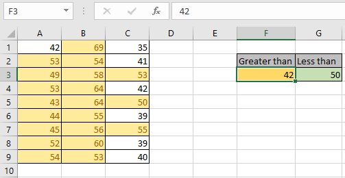 474×245 perform conditional formatting based cell excel from www.exceltip.com
 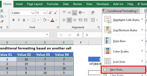 623×323 conditional formatting based cell excel google sheets from www.automateexcel.com
 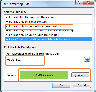 390×374 excel conditional formatting based column from www.exceltip.com
  619×587 conditional formatting based cell learn apply from www.educba.com
 How To Do Conditional Formatting Based On Another Cell In Excel was posted in July 17, 2025 at 6:16 am. If you wanna have it as yours, please click the Pictures and you will go to click right mouse then Save Image As and Click Save and download the How To Do Conditional Formatting Based On Another Cell In Excel Picture.. Don’t forget to share this picture with others via Facebook, Twitter, Pinterest or other social medias! we do hope you'll get inspired by ExcelKayra... Thanks again! If you have any DMCA issues on this post, please contact us!