How To Create A Dashboard With Pivot Charts In Excel
How To Create A Dashboard With Pivot Charts In Excel - There are a lot of affordable templates out there, but it can be easy to feel like a lot of the best cost a amount of money, require best special design template. Making the best template format choice is way to your template success. And if at this time you are looking for information and ideas regarding the How To Create A Dashboard With Pivot Charts In Excel then, you are in the perfect place. Get this How To Create A Dashboard With Pivot Charts In Excel for free here. We hope this post How To Create A Dashboard With Pivot Charts In Excel inspired you and help you what you are looking for.
“`html
Creating Interactive Dashboards with Pivot Charts in Excel
Excel dashboards are powerful tools for visualizing and analyzing data, providing a concise and dynamic overview of key performance indicators (KPIs). Pivot charts, built upon pivot tables, offer an excellent way to create interactive and easily customizable dashboard elements. This guide provides a step-by-step walkthrough on how to build a dashboard using pivot charts in Excel.
1. Prepare Your Data
The first and most crucial step is ensuring your data is well-structured and clean. A well-organized dataset makes creating pivot tables and charts significantly easier.
- Column Headers: Each column should have a clear and descriptive header. Avoid using abbreviations or jargon unless absolutely necessary.
- Consistent Data Types: Ensure that data within each column has a consistent data type (e.g., numbers, text, dates). Inconsistencies can lead to errors in pivot table calculations.
- No Empty Rows or Columns: Avoid leaving empty rows or columns within your data range, as this can interfere with pivot table recognition.
- Consistent Formatting: Format dates, numbers, and currency consistently throughout your dataset.
Example: Imagine you have sales data with columns like “Date,” “Product,” “Region,” “Salesperson,” “Quantity Sold,” and “Revenue.” Each of these columns should be appropriately formatted (e.g., “Date” as a date format, “Quantity Sold” as a number, and “Revenue” as currency).
2. Create Pivot Tables and Charts
Once your data is prepared, you can start creating pivot tables and their corresponding charts.
- Select Your Data: Click anywhere within your data range.
- Insert PivotTable: Go to the “Insert” tab on the Excel ribbon and click “PivotTable.”
- Choose Data Source and Location: A dialog box will appear. Verify the selected data range is correct. Choose whether to place the pivot table in a “New Worksheet” or an “Existing Worksheet.” Creating a new worksheet dedicated to pivot tables and charts is recommended for better organization.
- Build Your Pivot Table: The PivotTable Fields pane will appear on the right. Drag and drop fields from the list into the following areas:
- Rows: Fields placed here will appear as rows in the pivot table.
- Columns: Fields placed here will appear as columns in the pivot table.
- Values: Fields placed here will be summarized (e.g., sum, average, count).
- Filters: Fields placed here can be used to filter the data displayed in the pivot table.
- Create the Pivot Chart: With the pivot table selected, go to the “Insert” tab and choose a chart type (e.g., column chart, bar chart, line chart, pie chart) from the “Charts” group. Excel will automatically create a pivot chart linked to your pivot table.
Example: To analyze revenue by region, drag “Region” to the “Rows” area and “Revenue” to the “Values” area. Excel will automatically calculate the sum of revenue for each region. Then, create a column chart to visualize this data. Repeat this process to create pivot tables and charts for other KPIs like sales by product, quantity sold over time, etc.
3. Customize Pivot Charts
Pivot charts often require customization to improve readability and clarity.
- Chart Titles and Axis Labels: Double-click on the chart title and axis labels to edit them. Use descriptive and concise titles that clearly indicate what the chart is showing.
- Data Labels: Add data labels to display the values directly on the chart. This can be helpful for quickly identifying specific data points. Right-click on the chart and select “Add Data Labels.”
- Chart Styles and Colors: Use the “Chart Design” tab to change the chart style, colors, and fonts to match your dashboard’s overall theme. Consider using a consistent color palette for all charts.
- Axis Formatting: Adjust the axis scales, number formatting, and gridlines to enhance readability. Right-click on an axis and select “Format Axis.”
- Filter Buttons: Hide or customize the filter buttons on the chart if they are not needed for interaction on the dashboard itself. Right-click on a filter button and select “Hide Field Buttons on Chart” or “Remove Field.” You’ll likely want to retain these on at least one pivot table for the purpose of slicers.
- Sort Data: Sort your pivot table data for your graph to display in descending or ascending order. This can greatly improve quick comprehension of information.
4. Create a Dashboard Sheet
Create a new worksheet specifically for your dashboard. This sheet will house all your pivot charts and other elements.
- Rename the Sheet: Rename the sheet to something descriptive like “Dashboard” or “Sales Overview.”
- Remove Gridlines: Hide the gridlines on the dashboard sheet to create a cleaner look. Go to the “View” tab and uncheck “Gridlines.”
- Adjust Column Widths and Row Heights: Adjust column widths and row heights to create space for your charts and other dashboard elements.
5. Arrange and Format Dashboard Elements
Copy and paste your customized pivot charts from their individual worksheets to the dashboard sheet. Arrange them in a logical and visually appealing manner. Consider the following guidelines:
- Logical Layout: Arrange charts in a way that tells a story. Place the most important KPIs at the top and left of the dashboard, as these are the areas that users typically focus on first.
- Consistent Spacing: Maintain consistent spacing between charts to create a professional and organized look.
- Grouping: Group related charts together using borders or background colors to visually connect them.
- Branding: Incorporate your company’s logo and colors to reinforce brand identity.
6. Add Slicers and Timelines for Interactivity
Slicers and timelines are interactive controls that allow users to filter the data displayed in your pivot charts. Slicers are used to filter by categories, while timelines are used to filter by dates.
- Select a Pivot Table: Click on any of your pivot tables.
- Insert Slicer: Go to the “Analyze” (or “PivotTable Analyze” in some versions) tab and click “Insert Slicer.”
- Choose Fields for Slicers: Select the fields you want to use as slicers (e.g., “Region,” “Product,” “Salesperson”).
- Insert Timeline (for Date Fields): If you have a date field, click “Insert Timeline” and select the date field.
- Connect Slicers to Pivot Tables: Select a slicer. Go to the “Slicer” tab and click “Report Connections.” Check the boxes next to all the pivot tables you want the slicer to control. Repeat this process for each slicer and timeline. This ensures that all the charts on your dashboard update when you select a slicer value.
Example: If you create a slicer for “Region,” clicking on a specific region in the slicer will filter all the pivot charts on the dashboard to only show data for that region.
7. Enhance Dashboard Functionality (Optional)
- Calculated Fields and Items: Add calculated fields or items to your pivot tables to create new metrics or categories based on your existing data. This allows you to derive insights that are not directly available in your source data.
- Conditional Formatting: Use conditional formatting to highlight important data points or trends in your pivot tables. For example, you can use color scales to highlight high-performing regions or products.
- Macros (Advanced): For more advanced functionality, you can use macros to automate tasks, such as refreshing the data or changing the chart type.
8. Test and Refine
Thoroughly test your dashboard to ensure it is working correctly and that the data is accurate. Click on the slicers and timelines to verify that the charts update as expected. Get feedback from users and make adjustments based on their suggestions.
9. Refresh Your Data
To keep your dashboard up-to-date, you need to refresh the data regularly. Go to the “Data” tab and click “Refresh All.” You can also set up automatic data refresh in Excel options.
Conclusion
Creating interactive dashboards with pivot charts in Excel is a powerful way to visualize and analyze data. By following these steps, you can build a dynamic and informative dashboard that provides valuable insights for decision-making. Remember to focus on data preparation, chart customization, and interactive elements to create a user-friendly and effective dashboard.
“`
 1280×720 build dynamic interactive dashboard excel pivot tables from www.pinterest.com
  680×333 create professional excel dashboardpivot tables charts hwanjiku from www.fiverr.com
  3124×1506 create interactive excel dashboard pivot table charts vrogueco from www.vrogue.co
  680×364 survey feedback analysis excel share report qasim from www.fiverr.com
  649×348 create dynamic excel pivot table dashboard chart excel from www.exceldashboardtemplates.com
  680×411 create dashboard charts pivot tables excel alrohani fiverr from www.fiverr.com
  680×383 create excel dashboard charts reports pivot tables devanshi from www.fiverr.com
  1792×1024 create dashboard pivot chart excel from exceltemplatesforbusiness.com
  680×383 create dashboard charts pivot tables excel lateshmunde fiverr from www.fiverr.com
  1280×720 create excel dashboard pivot table charts data visualization from www.pixazsexy.com
  1280×720 interactive excel dashboard pivot table charts data hot sex from www.hotzxgirl.com
  680×513 create excel dashboard pivot table charts formulas data from www.fiverr.com
  680×390 create dynamic excel dashboard charts pivot tables macros from www.fiverr.com
  1000×493 create professional dashboard pivot tables charts vrogueco from www.vrogue.co
  680×494 create excel dashboard pivot tables charts muneebnasir from www.fiverr.com
  800×450 creating excel pivot table dashboard curiouscom from curious.com
  680×351 develop professional excel dashboardpivot tables charts from www.fiverr.com
  1280×720 build designed interactive excel dashboard pivot from quadexcel.com
  1280×720 excel pivot table dashboard excel dashboard templates class exam from www.myxxgirl.com
  1000×750 excel dashboard excel formula pivot tables power pivot upwork from www.upwork.com
  1248×725 conditions create pivot table lady excel from ladyexcel.com
  1000×750 interactive excel dashboard pivot table charts data visualization from www.upwork.com
  1306×740 dashboard pivottable business academics view from excelprof.com
 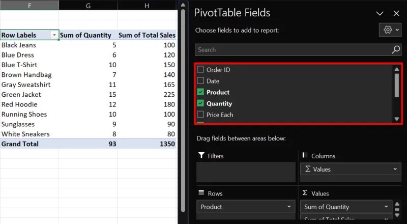 800×440 create excel dashboard tech easier from www.maketecheasier.com
  660×440 create interactive excel dashboard pivot table chart kpi from kwork.com
  680×325 pivot chart advance excel dashboard vijaysingh from www.fiverr.com
  1000×750 dynamic excel dashboard custom pivot tables charts graphs from www.upwork.com
  1000×750 interactive dashboard pivot table charts graphs reports excel from www.upwork.com
 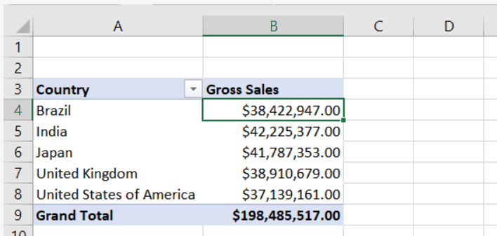 708×337 create dashboard excel earn excel from earnandexcel.com
  680×510 create excel dashboards pivot table charts maikdanyal fiverr from www.fiverr.com
  660×440 create excel dashboards graphs pivot tables charts from kwork.com
 How To Create A Dashboard With Pivot Charts In Excel was posted in June 1, 2025 at 11:04 am. If you wanna have it as yours, please click the Pictures and you will go to click right mouse then Save Image As and Click Save and download the How To Create A Dashboard With Pivot Charts In Excel Picture.. Don’t forget to share this picture with others via Facebook, Twitter, Pinterest or other social medias! we do hope you'll get inspired by ExcelKayra... Thanks again! If you have any DMCA issues on this post, please contact us!