How To Handle Errors Using Iferror Function In Excel Formulas

How To Handle Errors Using Iferror Function In Excel Formulas - There are a lot of affordable templates out there, but it can be easy to feel like a lot of the best cost a amount of money, require best special design template. Making the best template format choice is way to your template success. And if at this time you are looking for information and ideas regarding the How To Handle Errors Using Iferror Function In Excel Formulas then, you are in the perfect place. Get this How To Handle Errors Using Iferror Function In Excel Formulas for free here. We hope this post How To Handle Errors Using Iferror Function In Excel Formulas inspired you and help you what you are looking for.

Handling Errors with IFERROR in Excel

Excel is a powerful tool for data analysis and manipulation, but sometimes formulas can return errors. These errors, such as #DIV/0!, #VALUE!, #NAME?, #REF!, #NUM!, #N/A, and #NULL!, can disrupt your spreadsheets and make it difficult to interpret your results. The IFERROR function is a valuable tool for gracefully handling these errors, allowing you to replace them with more meaningful values or messages, thereby improving the clarity and usability of your spreadsheets.

Understanding the IFERROR Function

The IFERROR function takes two arguments:

1. value: This is the expression or formula that you want to evaluate.
2. value_if_error: This is the value you want to return if the first argument (value) results in an error.

The syntax is simple:

=IFERROR(value, value_if_error)

The function works as follows:

• If value evaluates successfully (i.e., does not return an error), IFERROR returns the result of value.
• If value results in any Excel error (e.g., #DIV/0!, #VALUE!), IFERROR returns value_if_error.

Common Excel Errors and How IFERROR Can Help

Here are some common Excel errors and how IFERROR can be used to address them:

1. #DIV/0! (Division by Zero)

This error occurs when you try to divide a number by zero or an empty cell.

Example:

Suppose you have sales data in column A and the number of customers in column B. You want to calculate the average sales per customer in column C.

The formula in column C would be: =A1/B1

If cell B1 is empty or contains zero, the formula in C1 will return #DIV/0!.

Using IFERROR to handle this:

=IFERROR(A1/B1, 0)

This formula will now return 0 if B1 is zero or empty, instead of the #DIV/0! error. You can replace the 0 with any other suitable value, such as “N/A” (Not Applicable) or leave it blank (“”).

2. #VALUE! (Incorrect Argument Type)

This error occurs when a function expects a certain type of argument (e.g., a number) but receives a different type (e.g., text).

Example:

You’re trying to add two cells together, but one of the cells contains text.

=A1+B1

If A1 contains a number and B1 contains text, this formula will return #VALUE!.

Using IFERROR to handle this:

=IFERROR(A1+B1, "")

This formula will return an empty string if either A1 or B1 contains text, preventing the #VALUE! error.

3. #NAME? (Unrecognized Name)

This error occurs when Excel doesn’t recognize a name used in your formula. This can happen if you misspell a function name or refer to a named range that doesn’t exist.

Example:

You accidentally type =SUMM(A1:A10) instead of =SUM(A1:A10).

This will result in a #NAME? error because “SUMM” is not a valid Excel function.

Using IFERROR to handle this:

While IFERROR can’t fix the underlying typo, it can prevent the error from displaying. However, in this case, it’s generally better to correct the formula than to mask the error with IFERROR, as it hides a fundamental mistake.

Still, for illustrative purposes:

=IFERROR(SUMM(A1:A10), "Check Formula")

This will display “Check Formula” instead of #NAME?. However, you should **always** fix the formula in this situation.

4. #REF! (Invalid Cell Reference)

This error occurs when a formula refers to a cell that is no longer valid, for example, if you delete a column or row that a formula references.

Example:

Your formula =SUM(A1:A10) refers to cells A1 to A10. If you delete column A, the formula will change to =SUM(#REF!:J10) and return #REF!.

Using IFERROR to handle this:

Similar to #NAME?, using IFERROR isn’t the ideal solution here. It’s better to revise the formula to use valid cell references. Masking this error will hide a potentially serious problem in your spreadsheet.

For illustrative purposes:

=IFERROR(SUM(A1:A10), "Reference Error")

This will display “Reference Error” if the reference becomes invalid, but it’s **crucial** to fix the formula.

5. #NUM! (Numeric Problem)

This error occurs when a formula has a problem with a number, such as trying to calculate the square root of a negative number without using complex numbers.

Example:

=SQRT(-1)

This will return #NUM! because the square root of a negative number is not a real number.

Using IFERROR to handle this:

=IFERROR(SQRT(-1), "Invalid Input")

This will display “Invalid Input” instead of #NUM!.

6. #N/A (Value Not Available)

This error is often used to indicate that a value is missing or not applicable. It’s frequently used with lookup functions like VLOOKUP, HLOOKUP, INDEX, and MATCH.

Example:

You’re using VLOOKUP to find a product’s price in a table, but the product code isn’t found in the lookup table.

=VLOOKUP("NonExistentProduct", A1:B10, 2, FALSE)

This will return #N/A because “NonExistentProduct” is not in the first column of the range A1:B10.

Using IFERROR to handle this:

=IFERROR(VLOOKUP("NonExistentProduct", A1:B10, 2, FALSE), "Product Not Found")

This will display “Product Not Found” if the VLOOKUP fails to find the product.

7. #NULL! (Intersection of Two Areas that Do Not Intersect)

This error is less common. It appears when you specify an intersection of two ranges that do not actually intersect.

Example:

=SUM(A1:A10 B1:B10) (Note the space between the ranges. A space used in a formula implies an intersection.)

If the intention was to sum both ranges separately, this formula is incorrect. Since the ranges A1:A10 and B1:B10 don’t intersect, it returns #NULL!.

Using IFERROR to handle this:

As with #NAME? and #REF!, fixing the formula is paramount. Using IFERROR masks a fundamental error.

For illustrative purposes:

=IFERROR(SUM(A1:A10 B1:B10), "No Intersection")

This will display “No Intersection”, but the **correct solution** is to use =SUM(A1:A10, B1:B10) or =SUM(A1:A10)+SUM(B1:B10) if you intended to sum both ranges.

Best Practices for Using IFERROR

• Use it Judiciously: Don’t use IFERROR as a substitute for fixing underlying formula errors. It’s best used to handle expected errors in situations where the input data might be incomplete or variable.
• Be Specific: Consider using other error-handling functions like ISERROR, ISERR, ISNA, etc., in conjunction with IF statements to handle specific error types if you need different responses for different errors. For instance, you might want to handle #N/A errors differently from #DIV/0! errors.
• Provide Informative Messages: Instead of just returning a blank cell or a generic “Error” message, provide informative messages that help users understand why the error occurred and what they can do to fix it.
• Test Your Formulas: Thoroughly test your formulas with various input values to ensure that IFERROR handles all potential error scenarios correctly.
• Consider Performance: While IFERROR is generally efficient, excessive use in complex spreadsheets can slightly impact performance. Evaluate if alternative approaches, such as cleaning your data beforehand, might be more efficient.

Nesting IFERROR Functions

You can nest IFERROR functions to handle multiple potential errors within a single formula. However, be cautious not to make your formulas overly complex, as this can make them difficult to understand and debug.

Example:

=IFERROR(VLOOKUP(A1, DataRange, 2, FALSE), IFERROR(INDEX(AltDataRange, MATCH(A1, AltLookupColumn, 0), 2), "Not Found"))

This formula first attempts a VLOOKUP. If that fails (returns an error), it tries an INDEX/MATCH combination as an alternative lookup method. If both fail, it returns “Not Found”.

Conclusion

The IFERROR function is an indispensable tool for creating robust and user-friendly Excel spreadsheets. By strategically using IFERROR, you can prevent error messages from disrupting your calculations and provide clear and informative feedback to users, ultimately leading to more reliable and understandable data analysis.

1281×662 excel iferror function excelfind from excelfind.com

474×260 ms excel iferror function ws from www.techonthenet.com

774×515 iferror function excel from www.exceltip.com

622×182 excel iferror function excel vba from www.exceldome.com

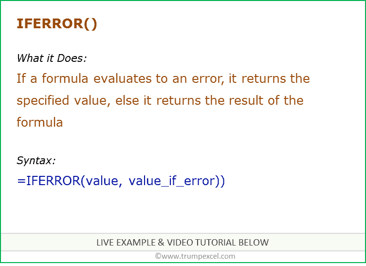752×546 excel iferror function formula examples video from trumpexcel.com

700×400 excel iferror function exceljet from exceljet.net

876×717 iferror function excel remove excel error excel unlocked from excelunlocked.com

767×702 iferror function excel examples exceldemy from www.exceldemy.com

1170×1200 iferror professor excel professor excel from professor-excel.com

649×437 iferror function excel efinancialmodels from www.efinancialmodels.com

735×499 handle errors excel iferror function examples from www.wallstreetmojo.com

1100×514 iferror function excel examples geeksforgeeks from www.geeksforgeeks.org

How To Handle Errors Using Iferror Function In Excel Formulas was posted in March 25, 2026 at 9:49 pm. If you wanna have it as yours, please click the Pictures and you will go to click right mouse then Save Image As and Click Save and download the How To Handle Errors Using Iferror Function In Excel Formulas Picture.. Don’t forget to share this picture with others via Facebook, Twitter, Pinterest or other social medias! we do hope you'll get inspired by ExcelKayra... Thanks again! If you have any DMCA issues on this post, please contact us!

Related For How To Handle Errors Using Iferror Function In Excel Formulas

Home Project Planner Excel With Tas

Home Project Planner in Excel: Mastering Task Assignments for

How to Use Excel Templates for Home

A home renovation model template is a pre-designed framework

Using A Corporate Tax Calculator To

How to Calculate Corporation Tax goselfemployed.co from goselfemployed.co Using

Create Stunning Charts with Chart T

Chart Templates Excel: The Ultimate Tool for Data Visualization