Home » Excel Templates » How To Use Conditional Formatting To Highlight Duplicates In Excel

How To Use Conditional Formatting To Highlight Duplicates In Excel

Wednesday, February 4th 2026. | Excel Templates

How To Use Conditional Formatting To Highlight Duplicates In Excel - There are a lot of affordable templates out there, but it can be easy to feel like a lot of the best cost a amount of money, require best special design template. Making the best template format choice is way to your template success. And if at this time you are looking for information and ideas regarding the How To Use Conditional Formatting To Highlight Duplicates In Excel then, you are in the perfect place. Get this How To Use Conditional Formatting To Highlight Duplicates In Excel for free here. We hope this post How To Use Conditional Formatting To Highlight Duplicates In Excel inspired you and help you what you are looking for.

find highlight remove duplicates excel

“`html

Highlighting Duplicates in Excel with Conditional Formatting

Excel’s conditional formatting feature is a powerful tool that allows you to automatically apply formatting to cells based on specific criteria. One common use is to highlight duplicate entries within a dataset. This is incredibly useful for data cleaning, identifying errors, and ensuring data integrity. This guide provides a comprehensive overview of how to use conditional formatting to highlight duplicates in Excel.

Why Highlight Duplicates?

Identifying and highlighting duplicates is crucial in various scenarios:

Data Cleaning: Removing or correcting duplicate data is essential for accurate analysis and reporting.
Error Detection: Duplicates can indicate data entry errors, system glitches, or inconsistencies.
Inventory Management: Identifying duplicate product IDs can prevent ordering errors and optimize stock levels.
Customer Relationship Management (CRM): Finding duplicate customer records allows for consolidating information and improving communication.
Financial Analysis: Detecting duplicate transactions can help identify fraudulent activity or accounting errors.

Methods for Highlighting Duplicates in Excel

Excel offers several methods for highlighting duplicates using conditional formatting. We’ll explore the most common and effective techniques.

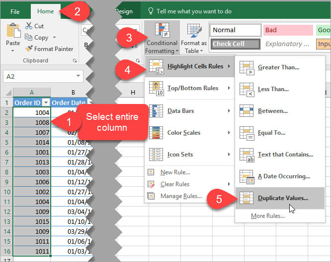
1. Using the Built-in “Highlight Cells Rules” > “Duplicate Values” Option

This is the simplest and most straightforward method for highlighting duplicates in a single column or range.

Select the Range: Select the column or range of cells you want to check for duplicates. For example, if you want to check column A, select all the data in column A (e.g., by clicking the column header “A”).
Access Conditional Formatting: Go to the “Home” tab in the Excel ribbon. In the “Styles” group, click on “Conditional Formatting.”
Choose “Highlight Cells Rules”: From the dropdown menu, select “Highlight Cells Rules.”
Select “Duplicate Values…”: In the submenu, choose “Duplicate Values…”
Customize the Formatting: A “Duplicate Values” dialog box will appear.
- The default setting highlights “Duplicate” values. You can also choose to highlight “Unique” values if needed.
- Use the “with” dropdown to select the formatting style you want to apply to the duplicate cells. You can choose from predefined styles like “Light Red Fill with Dark Red Text,” “Yellow Fill with Dark Yellow Text,” “Green Fill with Dark Green Text,” etc.
- To create a custom format, select “Custom Format…” from the dropdown. This opens the “Format Cells” dialog box, where you can customize the font, border, fill, and number formats.
Click “OK”: Click “OK” in both the “Format Cells” and “Duplicate Values” dialog boxes to apply the conditional formatting.

Now, any duplicate values within the selected range will be highlighted according to the formatting you specified.

2. Highlighting Duplicates Across Multiple Columns (Based on a Combination of Values)

Sometimes, a duplicate isn’t just based on a single cell’s value. You might need to identify duplicates based on a combination of values across multiple columns. For example, you might consider a record a duplicate if both the “FirstName” and “LastName” columns have the same values.

Select the Entire Data Range: Select the entire data range containing the columns you want to consider for duplication. This is important to ensure that the formatting is applied consistently across all rows.
Access Conditional Formatting: Go to the “Home” tab in the Excel ribbon. In the “Styles” group, click on “Conditional Formatting.”
Choose “New Rule…”: From the dropdown menu, select “New Rule…”
Select “Use a formula to determine which cells to format”: In the “New Formatting Rule” dialog box, select “Use a formula to determine which cells to format.”
Enter the Formula: In the formula box, enter a formula that identifies duplicate rows based on the combined values. The key is to use the COUNTIFS function.
The COUNTIFS function counts the number of cells that meet multiple criteria. The general syntax is:

=COUNTIFS(range1, criteria1, range2, criteria2, ...)

Here’s how to apply it to duplicate highlighting. Assuming your data starts in row 2 and you have “FirstName” in column A and “LastName” in column B, your formula would look like this:

=COUNTIFS($A:$A, $A2, $B:$B, $B2)>1
- $A:$A and $B:$B are the ranges containing the “FirstName” and “LastName” columns respectively. The dollar signs ($) before the column letters make these references absolute, meaning they won’t change when the formula is applied to other rows. Crucially, there are *no* dollar signs before the row number ‘2’ in `$A2` and `$B2`. This makes the criteria *relative* to the current row.
- $A2 and $B2 are the criteria for counting. They refer to the “FirstName” and “LastName” values in the *current row*. Excel will automatically adjust the row number as it applies the formula to each row.
- >1 checks if the count is greater than 1. If the count is greater than 1, it means that there is at least one other row with the same “FirstName” and “LastName” combination.
Set the Formatting: Click the “Format…” button to choose the formatting style you want to apply to the duplicate rows. This opens the “Format Cells” dialog box.
Choose Font, Border, and Fill Options: In the “Format Cells” dialog box, you can customize the font, border, and fill colors to highlight the duplicates. A common choice is to use a distinct fill color.
Click “OK”: Click “OK” in the “Format Cells” and “New Formatting Rule” dialog boxes to apply the conditional formatting.

Now, Excel will highlight entire rows where the combination of “FirstName” and “LastName” matches another row in the dataset.

3. Using Helper Columns (An Alternative Approach)

While conditional formatting with formulas is powerful, sometimes a helper column can make things more transparent and easier to manage, especially for complex scenarios or when troubleshooting.

Create a Helper Column: Insert a new column next to the columns you want to check for duplicates. This column will contain a formula that identifies duplicate rows. For example, if you want to check “FirstName” (Column A) and “LastName” (Column B), insert a new column C.
Enter the Formula in the Helper Column: In the first cell of the helper column (e.g., C2), enter a formula that combines the values from the relevant columns and then checks for duplicates using COUNTIFS. The formula would be: =IF(COUNTIFS($A:$A, $A2, $B:$B, $B2)>1, "Duplicate", "")
This formula works similarly to the conditional formatting formula but instead of applying formatting, it writes “Duplicate” if a duplicate is found and leaves the cell blank otherwise.
Drag the Formula Down: Drag the fill handle (the small square at the bottom-right corner of the cell) down to apply the formula to all rows in your data.
Apply Conditional Formatting to the Entire Data Range:
- Select the entire data range *including* the helper column.
- Go to “Home” > “Conditional Formatting” > “New Rule…”
- Select “Use a formula to determine which cells to format.”
- Enter the following formula: =$C2="Duplicate" (Assuming your helper column is column C, and the data starts on row 2). The dollar sign ensures that only the column letter will be fixed while it evaluates the rows.
- Set the formatting you want to apply to the duplicate rows.
- Click “OK”.

This method highlights entire rows where the helper column contains “Duplicate,” indicating that the combination of values in the “FirstName” and “LastName” columns is a duplicate.

Tips and Considerations

Data Types: Ensure that the data types in the columns you are comparing are consistent. For example, comparing text to numbers may lead to inaccurate results.
Case Sensitivity: By default, Excel’s duplicate detection is case-insensitive. To make it case-sensitive, use the EXACT function within your formulas. For example: =COUNTIFS($A:$A, EXACT($A2, $A:$A))>1
Leading and Trailing Spaces: Leading and trailing spaces can cause duplicates to be missed. Use the TRIM function to remove spaces before applying conditional formatting. For example: =COUNTIFS($A:$A, TRIM($A2), $B:$B, TRIM($B2))>1
Performance: Applying conditional formatting to very large datasets can slow down Excel. Consider using helper columns or filtering techniques for improved performance.
Remove Duplicates Feature: Excel also has a built-in “Remove Duplicates” feature (Data tab > Data Tools group). While this physically removes duplicates, highlighting them first allows you to review and verify the duplicates before deleting them.
Prioritize Your Criteria: Clearly define what constitutes a “duplicate” in your specific context. Is it an exact match across all columns, or a combination of key fields?

Conclusion

Conditional formatting is a versatile and efficient way to highlight duplicates in Excel. By understanding the different methods and considerations, you can effectively clean your data, identify errors, and ensure data integrity. Whether you choose the simple “Duplicate Values” rule or create more complex formulas, mastering these techniques will significantly improve your data analysis and reporting capabilities.

“`

666×529 filter duplicates conditional formatting excel campus from www.excelcampus.com

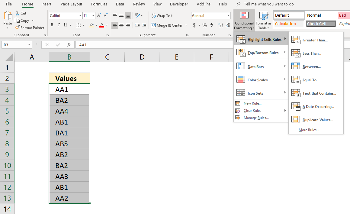1159×708 highlight uniqueduplicates conditional formatting from www.get-digital-help.com

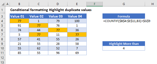654×267 highlight duplicate values excel google sheets automate excel from www.automateexcel.com

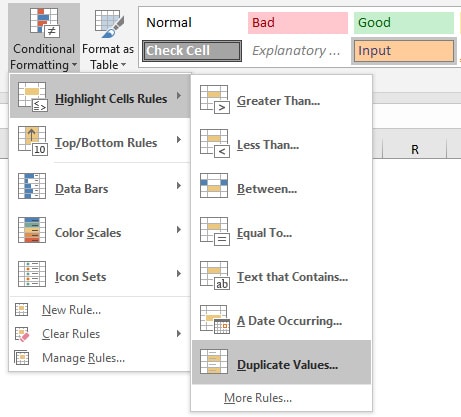461×417 find duplicates excel step step guide clean data from excelexplained.com

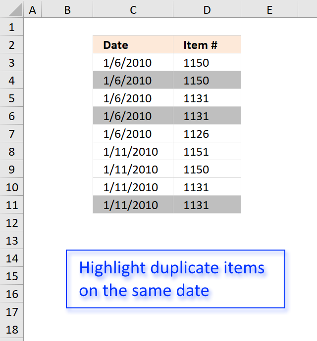474×431 excel conditional formatting highlight duplicates suppress empty from answers.microsoft.com

640×690 highlight duplicate values from www.get-digital-help.com

420×293 highlight duplicates excel examples highlight duplicates from www.educba.com

630×488 find highlight remove duplicates excel from www.exceldemy.com

640×384 highlight duplicates microsoft excel from www.groovypost.com

How To Use Conditional Formatting To Highlight Duplicates In Excel was posted in February 4, 2026 at 5:43 am. If you wanna have it as yours, please click the Pictures and you will go to click right mouse then Save Image As and Click Save and download the How To Use Conditional Formatting To Highlight Duplicates In Excel Picture.. Don’t forget to share this picture with others via Facebook, Twitter, Pinterest or other social medias! we do hope you'll get inspired by ExcelKayra... Thanks again! If you have any DMCA issues on this post, please contact us!