How To Insert Checkboxes In Excel For Interactive Task Lists
How To Insert Checkboxes In Excel For Interactive Task Lists - There are a lot of affordable templates out there, but it can be easy to feel like a lot of the best cost a amount of money, require best special design template. Making the best template format choice is way to your template success. And if at this time you are looking for information and ideas regarding the How To Insert Checkboxes In Excel For Interactive Task Lists then, you are in the perfect place. Get this How To Insert Checkboxes In Excel For Interactive Task Lists for free here. We hope this post How To Insert Checkboxes In Excel For Interactive Task Lists inspired you and help you what you are looking for.
“`html
Creating Interactive Task Lists in Excel with Checkboxes
Excel can be much more than just a spreadsheet for numbers; it can be a powerful tool for project management and task tracking. One of the most effective ways to make your Excel task lists interactive is by using checkboxes. Checkboxes allow you to visually mark tasks as complete, instantly updating the list’s status and potentially triggering other actions within your spreadsheet. This guide will walk you through the process of inserting and utilizing checkboxes in Excel for creating dynamic and engaging task lists.
Enabling the Developer Tab
Before you can insert checkboxes, you need to ensure the “Developer” tab is visible in your Excel ribbon. By default, it’s hidden. Here’s how to enable it:
- Click the File tab.
- Click Options.
- In the Excel Options dialog box, click Customize Ribbon.
- In the right-hand pane, under “Customize the Ribbon,” find the Developer checkbox.
- Check the Developer box.
- Click OK.
The “Developer” tab should now appear in your Excel ribbon.
Inserting Checkboxes
With the Developer tab enabled, you can now insert checkboxes into your worksheet. Here’s the step-by-step process:
- Click the Developer tab.
- In the “Controls” group, click Insert.
- Under “Form Controls,” select the Checkbox (Form Control) option. It’s usually the first icon in the top row.
- Click and drag on your worksheet to draw the checkbox. The size of the rectangle you draw will determine the size of the checkbox. Aim for a size that fits comfortably in your cells.
- Edit the Text: By default, the checkbox will be labeled something like “Check Box 1.” Click on the text next to the checkbox (not the checkbox itself) and delete it. You usually want the checkbox to appear directly next to the task description.
- Position the Checkbox: Carefully drag the checkbox into the cell next to your task description. You may need to resize or reposition it to align it perfectly. Using the arrow keys after selecting the checkbox can help with fine-grained adjustments.
Linking Checkboxes to Cells
The real power of checkboxes comes from linking them to cells. This allows you to use the checkbox’s status (TRUE for checked, FALSE for unchecked) to drive other calculations, formatting, or actions in your spreadsheet. Here’s how to link a checkbox to a cell:
- Right-click on the checkbox.
- Select Format Control… from the context menu.
- In the “Format Control” dialog box, go to the Control tab.
- In the “Cell link” box, enter the cell reference where you want to store the checkbox’s value. For example, if the checkbox is in cell B2 and you want to link it to cell C2, enter “C2” in the box. You can also click the small spreadsheet icon next to the box to select the cell directly.
- Click OK.
Now, when you check or uncheck the box, the linked cell will display TRUE or FALSE, respectively. You can then use this TRUE/FALSE value in formulas or conditional formatting.
Creating a Task List and Linking Checkboxes
Let’s create a simple task list and link checkboxes to it:
- In column A, enter your task descriptions. For example:
- A1: Write Report
- A2: Schedule Meeting
- A3: Review Documents
- In column B, insert a checkbox next to each task, following the steps outlined above.
- Link each checkbox to a cell in column C. For example:
- Link the checkbox in B1 to C1.
- Link the checkbox in B2 to C2.
- Link the checkbox in B3 to C3.
Now, when you check a box in column B, the corresponding cell in column C will display TRUE. Unchecking the box will change the value to FALSE.
Using Checkbox Values for Conditional Formatting
One of the most common uses of linked checkboxes is to apply conditional formatting. This allows you to visually indicate when a task is complete, such as by changing the text color or filling the cell.
- Select the task descriptions in column A (A1:A3 in our example).
- Click the Home tab.
- In the “Styles” group, click Conditional Formatting.
- Select New Rule…
- In the “New Formatting Rule” dialog box, select “Use a formula to determine which cells to format.”
- In the “Format values where this formula is true” box, enter a formula that references the linked cell. For example, if the checkbox for “Write Report” (A1) is linked to C1, the formula would be `=C1=TRUE`. Similarly, for A2 it would be `=C2=TRUE`, and for A3, `=C3=TRUE`. You will need to create separate rules for each task to ensure the formula references the correct linked cell.
- Click the Format… button to choose the formatting you want to apply when the condition is true (i.e., when the checkbox is checked). You can change the font color, fill color, or apply other formatting options.
- Click OK to close the “Format Cells” dialog box.
- Click OK to close the “New Formatting Rule” dialog box.
Now, when you check a box, the corresponding task description will be formatted according to the rule you defined. For example, you could set the font color to gray and apply a strikethrough to indicate that the task is complete.
Counting Completed Tasks
You can use the linked cell values to count the number of completed tasks. Use the `COUNTIF` function:
`=COUNTIF(C1:C3, TRUE)`
This formula will count the number of cells in the range C1:C3 that contain the value TRUE (i.e., the number of checked checkboxes).
Calculating Task Completion Percentage
You can calculate the percentage of tasks completed by combining the `COUNTIF` function with the `COUNTA` function (which counts non-empty cells):
`=(COUNTIF(C1:C3, TRUE)/COUNTA(A1:A3))*100`
This formula divides the number of completed tasks (TRUE values in column C) by the total number of tasks (non-empty cells in column A) and multiplies by 100 to express the result as a percentage.
Copying Checkboxes
Copying checkboxes directly can sometimes be tricky. Instead of directly copying and pasting, consider using the “Format Painter” after you’ve created and linked your first checkbox.
- Create and link your first checkbox as described above.
- Select the cell containing the linked checkbox (e.g., B1).
- Click the Home tab.
- In the “Clipboard” group, click the Format Painter button.
- Click and drag down the cells where you want to create the remaining checkboxes (e.g., B2:B3).
- You’ll need to adjust the linked cells for each checkbox individually using the ‘Format Control’ dialogue box, as described earlier.
Advanced Tips and Considerations
- Grouping: If you have many checkboxes, consider grouping them together to manage them more easily. This can be done in the Developer tab, under the ‘Group’ option.
- Data Validation: You can use data validation to prevent users from entering invalid data in the cells linked to the checkboxes. This can help maintain the integrity of your task list.
- Macros: For more advanced functionality, you can use VBA macros to automate tasks related to the checkboxes, such as sending email notifications when a task is completed.
- Alternative Controls: Explore other form controls available in the Developer tab, such as Option Buttons and Combo Boxes, for different types of interactive elements in your spreadsheet.
- Accessibility: While checkboxes enhance interactivity, ensure your task list is still accessible to users with disabilities. Provide clear labels and consider using alternative methods for conveying information if necessary.
By following these steps, you can create interactive and visually appealing task lists in Excel that help you stay organized and track your progress effectively. The use of checkboxes, linked cells, and conditional formatting transforms a static spreadsheet into a dynamic tool for project management and personal productivity.
“`
 756×228 insert checkbox excel easy step step guide from trumpexcel.com
  452×398 insert checkbox excel from www.repairmsexcel.com
  740×356 insert checkbox excel create interactive lists charts from trumpexcel.com
 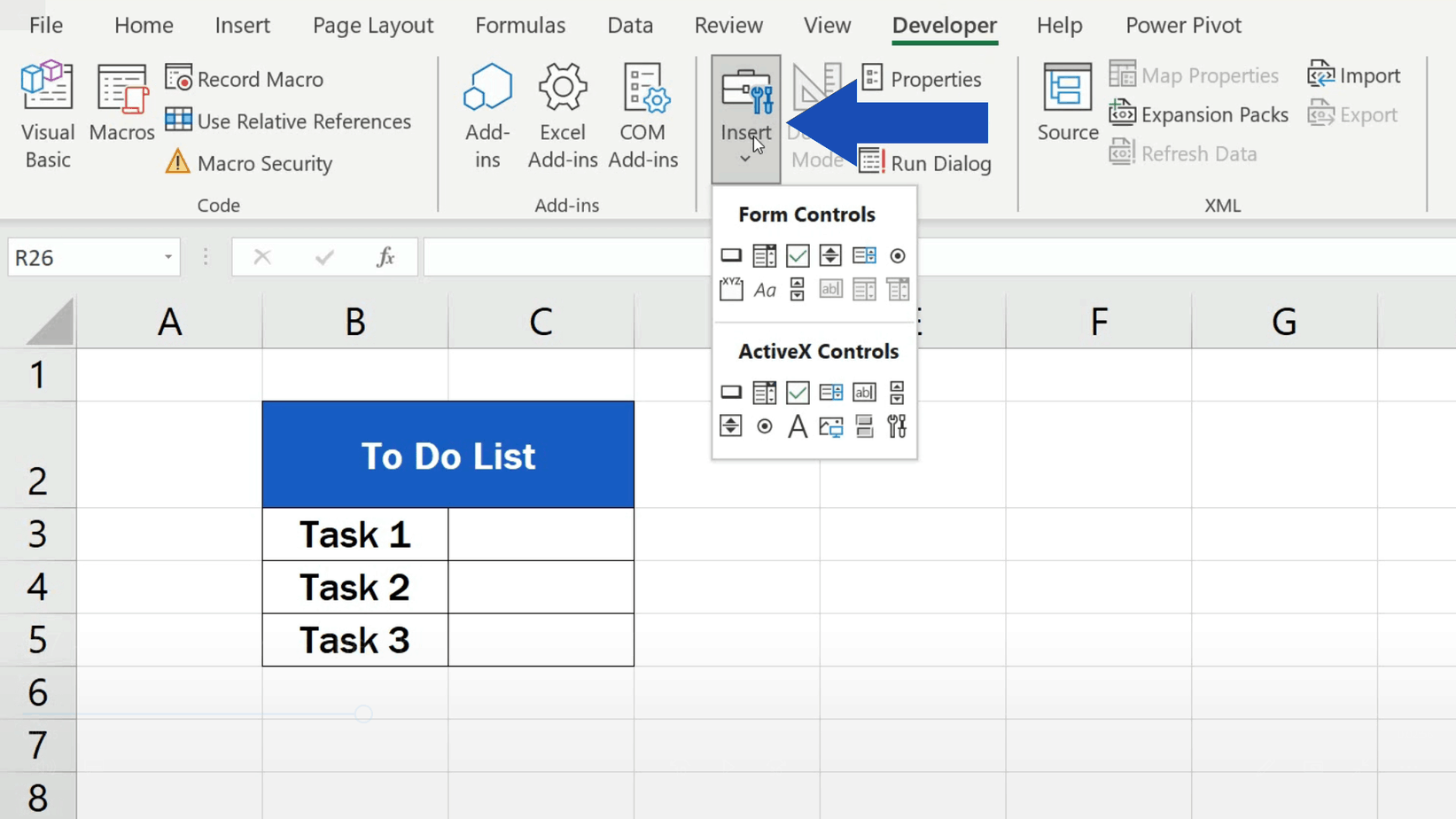 1643×924 insert checkbox excel from www.easyclickacademy.com
 How To Insert Checkboxes In Excel For Interactive Task Lists was posted in February 23, 2026 at 1:02 pm. If you wanna have it as yours, please click the Pictures and you will go to click right mouse then Save Image As and Click Save and download the How To Insert Checkboxes In Excel For Interactive Task Lists Picture.. Don’t forget to share this picture with others via Facebook, Twitter, Pinterest or other social medias! we do hope you'll get inspired by ExcelKayra... Thanks again! If you have any DMCA issues on this post, please contact us!