Excel Formula For Calculating Loan Interest Monthly
Excel Formula For Calculating Loan Interest Monthly - There are a lot of affordable templates out there, but it can be easy to feel like a lot of the best cost a amount of money, require best special design template. Making the best template format choice is way to your template success. And if at this time you are looking for information and ideas regarding the Excel Formula For Calculating Loan Interest Monthly then, you are in the perfect place. Get this Excel Formula For Calculating Loan Interest Monthly for free here. We hope this post Excel Formula For Calculating Loan Interest Monthly inspired you and help you what you are looking for.
“`html
Calculating Loan Interest Monthly in Excel
Understanding how to calculate the interest portion of your monthly loan payments is crucial for effective budgeting and financial planning. Excel offers several powerful functions to accomplish this accurately and efficiently. This guide will walk you through the key formulas and techniques to calculate loan interest on a monthly basis.
Key Excel Functions for Loan Calculations
Before diving into the specifics of interest calculation, let’s introduce the essential Excel functions you’ll need:
- PMT (Payment): Calculates the periodic payment for a loan. This function factors in the interest rate, loan term, and principal amount.
- IPMT (Interest Payment): Calculates the interest portion of a loan payment for a specific period.
- PPMT (Principal Payment): Calculates the principal portion of a loan payment for a specific period.
- RATE: Calculates the interest rate per period of a loan or investment.
- NPER (Number of Periods): Calculates the number of periods for a loan or investment.
- PV (Present Value): Calculates the present value (principal amount) of a loan or investment.
Calculating Monthly Interest with IPMT
The IPMT function is your primary tool for determining the interest portion of each monthly payment. The syntax for IPMT is as follows:
=IPMT(rate, per, nper, pv, [fv], [type])Let’s break down each argument:
- rate: The interest rate per period. Since we’re calculating monthly interest, you’ll need to divide the annual interest rate by 12. For example, if the annual interest rate is 6%, the monthly rate would be 6%/12 = 0.005.
- per: The period for which you want to calculate the interest. This is a number between 1 and the total number of periods (
nper). For example, to calculate the interest for the first month,perwould be 1. For the second month, it would be 2, and so on. - nper: The total number of payment periods for the loan. If the loan term is in years, you’ll need to multiply it by 12 to get the number of months. For example, a 5-year loan would have 5 * 12 = 60 periods.
- pv: The present value (or principal amount) of the loan. This is the initial amount borrowed.
- [fv]: (Optional) The future value of the loan after the last payment is made. If omitted, it’s assumed to be 0 (meaning the loan is fully paid off).
- [type]: (Optional) Specifies when payments are due. 0 indicates payments are due at the end of the period (most common), and 1 indicates payments are due at the beginning of the period. If omitted, it’s assumed to be 0.
Example: Calculating the Interest for the First Month
Let’s say you have a loan with the following characteristics:
- Principal (PV): $20,000
- Annual Interest Rate: 6%
- Loan Term: 5 years (60 months)
To calculate the interest portion of the first month’s payment, you would use the following formula in Excel:
=IPMT(6%/12, 1, 60, 20000)This formula calculates the interest for the first month (per=1) of a 60-month loan (nper=60) with a $20,000 principal (pv=20000) and an annual interest rate of 6% (rate=6%/12).
The result will be a negative number (e.g., -$100). The negative sign indicates an outflow of cash. You can use the ABS function to get the absolute value if you prefer a positive number:
=ABS(IPMT(6%/12, 1, 60, 20000))Creating an Amortization Schedule
To calculate the interest portion for each month of the loan, you can create an amortization schedule in Excel. This table will show the breakdown of each payment into its principal and interest components.
- Set up the headings: In the first row of your spreadsheet, create headings for: “Month,” “Payment,” “Interest,” “Principal,” and “Balance.”
- Enter the initial data: In the first row under the headings, enter the initial loan details. The “Month” will be 0, “Payment” will be blank (or 0), “Interest” will be blank, “Principal” will be blank, and “Balance” will be the principal amount of the loan (e.g., $20,000).
- Calculate the monthly payment: Use the
PMTfunction to calculate the fixed monthly payment. Enter the following formula in a separate cell (e.g., cell G1):=PMT(6%/12, 60, 20000)Make sure to reference this cell when calculating the “Payment” column in your amortization schedule (see below). Using cell references ensures the payment is consistent for each month.
- Populate the “Month” column: Enter 1 in the “Month” column for the second row. Then, in the cell below, enter the formula
=A2+1(assuming A2 is the cell containing “1”). Drag this formula down to create a sequence of months from 1 to 60. - Calculate “Payment”: In the “Payment” column (e.g., column B), enter the formula
=$G$1(assuming cell G1 contains the PMT formula from step 3). The$signs make it an absolute reference, so the formula will always refer to that cell when you drag it down. - Calculate “Interest”: In the “Interest” column (e.g., column C), enter the
IPMTformula, referencing the appropriate month:=IPMT(6%/12, A2, 60, D1)*
A2refers to the “Month” cell for that row. *6%/12is the monthly interest rate. *60is the total number of periods. *D1refers to the “Balance” from the *previous* month (important!). - Calculate “Principal”: In the “Principal” column (e.g., column D), enter the
PPMTformula, similarly referencing the appropriate month and balance:=PPMT(6%/12, A2, 60, D1)*
A2refers to the “Month” cell for that row. *6%/12is the monthly interest rate. *60is the total number of periods. *D1refers to the “Balance” from the *previous* month. - Calculate “Balance”: In the “Balance” column (e.g., column E), enter the formula to subtract the principal payment from the previous month’s balance:
=D1+D2*
D1refers to the previous month’s balance. *D2refers to the current month’s principal payment (remember principal payment will be a negative value, so adding it actually subtracts the value). - Copy the formulas: Select the cells containing the formulas for “Payment,” “Interest,” “Principal,” and “Balance” (from the second row). Drag the fill handle (the small square at the bottom-right corner of the selection) down to row 61 to populate the formulas for all 60 months.
Your amortization schedule will now show the breakdown of each payment into interest and principal, as well as the remaining balance after each payment. The “Balance” in the last row (month 60) should be very close to zero (any small difference is usually due to rounding errors).
Important Considerations
- Interest Rate Precision: Excel stores numbers with a high degree of precision. While you might only see two decimal places for the interest rate, Excel uses the full precision in its calculations. This is important for accurate results, especially over long loan terms.
- Rounding: Slight rounding differences can occur when manually calculating loan amortizations. Excel’s functions are generally very accurate, but you might still encounter minor discrepancies.
- Loan Type: These formulas are designed for fixed-rate loans with regular payment intervals. For variable-rate loans or loans with irregular payments, you’ll need more complex calculations.
Conclusion
Excel’s IPMT, PMT, and PPMT functions provide a powerful and efficient way to calculate loan interest and create amortization schedules. By understanding the arguments of these functions and following the steps outlined above, you can gain valuable insights into your loan payments and manage your finances more effectively.
“`
 700×400 excel formula calculate loan interest year exceljet from exceljet.net
 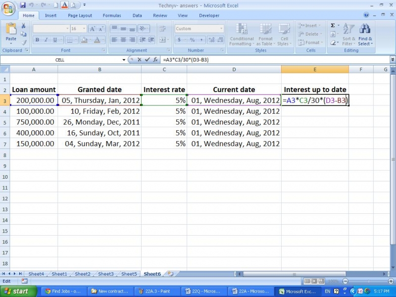 800×600 calculate loan interest date excel formula from www.techyv.com
  806×644 calculate monthly loan payments excel investinganswers from investinganswers.com
  2255×2190 loan amortization schedule spreadsheet db excelcom from db-excel.com
  696×229 calculate total interest paid loan formula wall art from www.vvengelbert.nl
  809×416 calculate interest payments period total excel formulas from www.extendoffice.com
  484×515 interest loan calculator excel from www.vertex42.com
  3200×2410 calculate interest payment excel easy steps from www.wikihow.com
 Excel Formula For Calculating Loan Interest Monthly was posted in January 23, 2026 at 8:33 am. If you wanna have it as yours, please click the Pictures and you will go to click right mouse then Save Image As and Click Save and download the Excel Formula For Calculating Loan Interest Monthly Picture.. Don’t forget to share this picture with others via Facebook, Twitter, Pinterest or other social medias! we do hope you'll get inspired by ExcelKayra... Thanks again! If you have any DMCA issues on this post, please contact us!