How To Calculate Asset Depreciation In Excel Using Straight-line Method
How To Calculate Asset Depreciation In Excel Using Straight-line Method - There are a lot of affordable templates out there, but it can be easy to feel like a lot of the best cost a amount of money, require best special design template. Making the best template format choice is way to your template success. And if at this time you are looking for information and ideas regarding the How To Calculate Asset Depreciation In Excel Using Straight-line Method then, you are in the perfect place. Get this How To Calculate Asset Depreciation In Excel Using Straight-line Method for free here. We hope this post How To Calculate Asset Depreciation In Excel Using Straight-line Method inspired you and help you what you are looking for.
“`html
Calculating Asset Depreciation in Excel Using the Straight-Line Method
Depreciation is the systematic allocation of the cost of an asset over its useful life. It reflects the gradual decline in the asset’s value due to wear and tear, obsolescence, or other factors. Accurately calculating depreciation is crucial for financial reporting, tax purposes, and internal decision-making. The straight-line method is one of the simplest and most commonly used depreciation methods. This method allocates an equal amount of depreciation expense each year over the asset’s useful life. This article explains how to calculate asset depreciation using the straight-line method in Microsoft Excel.
Understanding the Straight-Line Depreciation Method
The straight-line method is based on the assumption that an asset provides equal benefits throughout its useful life. Therefore, the depreciation expense is the same for each period. The formula for calculating straight-line depreciation is:
Annual Depreciation Expense = (Cost – Salvage Value) / Useful Life
- Cost: The original cost of the asset, including all expenses incurred to acquire and prepare the asset for its intended use.
- Salvage Value: The estimated value of the asset at the end of its useful life. This is also known as residual value.
- Useful Life: The estimated number of years (or periods) the asset will be used for its intended purpose.
Setting Up Your Excel Worksheet
Before diving into the formulas, it’s helpful to structure your Excel worksheet in a clear and organized manner. Consider using the following columns:
- Asset Name: A descriptive name for the asset (e.g., “Delivery Truck,” “Office Equipment”).
- Cost: The original cost of the asset.
- Salvage Value: The estimated salvage value of the asset.
- Useful Life (Years): The estimated useful life of the asset in years.
- Annual Depreciation: The annual depreciation expense calculated using the straight-line method.
- Accumulated Depreciation: The total depreciation expense recorded for the asset to date.
- Book Value: The asset’s cost less accumulated depreciation.
- Year: (Optional) A column representing each year of the asset’s useful life, allowing you to track depreciation expense year by year.
Here’s an example of how your worksheet might look:
| Asset Name | Cost | Salvage Value | Useful Life (Years) | Annual Depreciation | Accumulated Depreciation | Book Value | Year 1 | Year 2 | Year 3 |
|---|---|---|---|---|---|---|---|---|---|
| Delivery Truck | $50,000 | $5,000 | 5 | ||||||
| Office Equipment | $20,000 | $2,000 | 10 |
Calculating Annual Depreciation in Excel
Now, let’s calculate the annual depreciation expense using Excel formulas.
- Enter the Data: Input the Cost, Salvage Value, and Useful Life (Years) for each asset into their respective columns. For example, in the first row for the “Delivery Truck,” you’d enter $50,000 in the “Cost” column, $5,000 in the “Salvage Value” column, and 5 in the “Useful Life (Years)” column.
- Calculate Annual Depreciation: In the “Annual Depreciation” column, enter the following formula. Assuming the Cost is in cell B2, Salvage Value is in cell C2, and Useful Life is in cell D2, the formula in cell E2 would be:
=(B2-C2)/D2This formula subtracts the salvage value from the cost and then divides the result by the useful life. In our example, this would calculate to ($50,000 – $5,000) / 5 = $9,000. This means the annual depreciation expense for the delivery truck is $9,000.
- Copy the Formula: Drag the fill handle (the small square at the bottom-right corner of cell E2) down to apply the formula to other assets in your worksheet. Excel will automatically adjust the cell references to calculate the annual depreciation for each asset based on its cost, salvage value, and useful life.
Calculating Accumulated Depreciation and Book Value
Now that you have the annual depreciation, you can calculate the accumulated depreciation and book value for each year of the asset’s life. Let’s populate the ‘Year’ columns to demonstrate this.
- Year 1:
- Accumulated Depreciation (Year 1): In the “Accumulated Depreciation” column for Year 1 (for example, cell F2), simply enter the annual depreciation from column E:
=E2. This is because in the first year, the accumulated depreciation is equal to the annual depreciation expense. - Book Value (Year 1): The book value is the original cost minus the accumulated depreciation. Assuming the cost is in cell B2 and the accumulated depreciation (Year 1) is in cell F2, the formula for the Book Value in Year 1 (cell G2) would be:
=B2-F2. This is $50,000 – $9,000 = $41,000 for the Delivery Truck.
- Accumulated Depreciation (Year 1): In the “Accumulated Depreciation” column for Year 1 (for example, cell F2), simply enter the annual depreciation from column E:
- Year 2 and Subsequent Years:
- Accumulated Depreciation (Year 2 onwards): The accumulated depreciation for subsequent years is the accumulated depreciation from the previous year plus the annual depreciation. In the “Year 2” column (e.g., column H), you would place the annual depreciation again:
=E2. Then, to calculate the *total* Accumulated Depreciation *at the end* of Year 2 (cell F3 – note the row change!), you would use this formula:=F2+H2. This adds the prior year’s accumulated depreciation to the current year’s depreciation expense. - Book Value (Year 2 onwards): The book value is calculated as the original cost minus the *current* accumulated depreciation. So, the Book Value at the end of Year 2 (cell G3) would be:
=B2-F3.
- Accumulated Depreciation (Year 2 onwards): The accumulated depreciation for subsequent years is the accumulated depreciation from the previous year plus the annual depreciation. In the “Year 2” column (e.g., column H), you would place the annual depreciation again:
- Copy the Formulas: Drag the formulas for “Accumulated Depreciation” and “Book Value” down to apply them to other assets, and across to subsequent years. Remember to adjust the cell references accordingly to ensure you’re referencing the correct cells for each asset and year.
By the end of the asset’s useful life, the accumulated depreciation should equal the depreciable base (Cost – Salvage Value), and the book value should equal the salvage value.
Using Excel’s SLN Function (An Alternative Method)
Excel also provides a built-in function for calculating straight-line depreciation: the `SLN` function. The syntax is:
=SLN(cost, salvage, life)
- cost: The original cost of the asset.
- salvage: The salvage value of the asset.
- life: The useful life of the asset.
Using the `SLN` function is even simpler than creating the formula manually. In the “Annual Depreciation” column, you could use the following formula (assuming the Cost is in cell B2, Salvage Value is in cell C2, and Useful Life is in cell D2):
=SLN(B2,C2,D2)
This formula will directly calculate the annual depreciation expense for the asset. You can then proceed to calculate accumulated depreciation and book value as described in the previous sections.
Important Considerations
* Partial-Year Depreciation: If an asset is placed in service during the middle of a year, you may need to calculate partial-year depreciation. You can adjust the annual depreciation formula to reflect the portion of the year the asset was in service. For example, if an asset was placed in service on July 1st, you would multiply the annual depreciation by 6/12 (or 0.5) to calculate the depreciation expense for that year. * Depreciation Methods: The straight-line method is just one of several depreciation methods. Other methods, such as the double-declining balance method and the sum-of-the-years’ digits method, may be more appropriate for certain assets or situations. These methods result in higher depreciation expense in the early years of the asset’s life and lower depreciation expense in the later years. * Tax Regulations: Depreciation is subject to tax regulations that vary by jurisdiction. Consult with a tax professional to ensure you are using the correct depreciation method and complying with all applicable tax laws. * Regular Review: Periodically review the estimated useful life and salvage value of your assets to ensure they are still accurate. Changes in technology, market conditions, or the asset’s condition may warrant an adjustment to these estimates. * Error Checking: Always double-check your formulas and data inputs to ensure accuracy. Even small errors can have a significant impact on your financial statements.
Conclusion
Calculating asset depreciation using the straight-line method in Excel is a straightforward process. By following the steps outlined in this article, you can easily calculate annual depreciation expense, accumulated depreciation, and book value for your assets. Remember to consider the important considerations discussed above to ensure your depreciation calculations are accurate and compliant with applicable regulations. Excel’s built-in `SLN` function provides an even quicker way to calculate straight-line depreciation, but understanding the underlying formula is crucial for making informed decisions about asset management and financial reporting.
“`
 700×400 easily calculate straight depreciation excel exceldatapro from exceldatapro.com
  895×512 straight depreciation calculator from myexceltemplates.com
  800×348 straight depreciation definition formula accounting from exceldatapro.com
  634×643 straight depreciation schedule calculator double entry bookkeeping from www.double-entry-bookkeeping.com
  768×395 straight depreciation formula calculator excel template from www.educba.com
 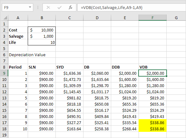 604×447 depreciation formulas excel complete tutorial from www.excel-easy.com
 How To Calculate Asset Depreciation In Excel Using Straight-line Method was posted in July 4, 2025 at 6:52 pm. If you wanna have it as yours, please click the Pictures and you will go to click right mouse then Save Image As and Click Save and download the How To Calculate Asset Depreciation In Excel Using Straight-line Method Picture.. Don’t forget to share this picture with others via Facebook, Twitter, Pinterest or other social medias! we do hope you'll get inspired by ExcelKayra... Thanks again! If you have any DMCA issues on this post, please contact us!