How To Calculate Depreciation Using Double Declining Balance In Excel
How To Calculate Depreciation Using Double Declining Balance In Excel - There are a lot of affordable templates out there, but it can be easy to feel like a lot of the best cost a amount of money, require best special design template. Making the best template format choice is way to your template success. And if at this time you are looking for information and ideas regarding the How To Calculate Depreciation Using Double Declining Balance In Excel then, you are in the perfect place. Get this How To Calculate Depreciation Using Double Declining Balance In Excel for free here. We hope this post How To Calculate Depreciation Using Double Declining Balance In Excel inspired you and help you what you are looking for.
Calculating Depreciation with the Double-Declining Balance Method in Excel
The double-declining balance (DDB) method is an accelerated depreciation method, meaning it recognizes more depreciation expense in the early years of an asset’s life and less in the later years. It’s a valuable tool for businesses wanting to quickly expense an asset’s cost. Excel provides a straightforward way to calculate DDB depreciation, making it easy to track asset values over time.
Understanding the Double-Declining Balance Method
Before diving into Excel, let’s briefly recap the DDB method. The basic formula is:
Depreciation Expense = 2 * (Book Value at Beginning of Year) * (Depreciation Rate)
Where:
- Book Value at Beginning of Year: This is the asset’s cost minus accumulated depreciation from previous years.
- Depreciation Rate: This is calculated as 1 / (Useful Life). The “double” in double-declining balance refers to multiplying this rate by 2.
- Useful Life: The estimated number of years the asset will be used.
A crucial aspect of the DDB method is that you don’t depreciate an asset below its salvage value. Salvage value is the estimated value of the asset at the end of its useful life. You must adjust the depreciation expense in the final year (or years) to ensure the book value doesn’t fall below the salvage value.
Using Excel’s DDB Function
Excel provides a dedicated `DDB` function to simplify the calculation. The syntax is:
=DDB(cost, salvage, life, period, [factor])
Let’s break down each argument:
- cost: The initial cost of the asset.
- salvage: The salvage value of the asset.
- life: The useful life of the asset in years.
- period: The specific period (year) for which you want to calculate depreciation. This is a number, usually starting from 1.
- [factor]: (Optional) The rate at which the balance declines. If omitted, it defaults to 2 (which is why it’s called *double* declining balance). You can adjust this if you want to use a different declining balance rate. For example, setting it to 1.5 would be a 150% declining balance.
Creating a Depreciation Schedule in Excel
Here’s how to create a complete depreciation schedule using the DDB function, including the critical adjustment for salvage value:
- Set up your data: In your Excel sheet, create columns for the following:
- Year: The year number (e.g., 1, 2, 3…).
- DDB Depreciation: The depreciation expense calculated by the DDB function.
- Accumulated Depreciation: The total depreciation taken up to and including that year.
- Book Value: The asset’s cost minus accumulated depreciation.
- Enter the asset’s details: In separate cells (e.g., A1, B1, C1), enter the following values:
- Cost: The asset’s initial cost (e.g., $10,000).
- Salvage Value: The asset’s estimated salvage value (e.g., $1,000).
- Useful Life: The asset’s useful life in years (e.g., 5).
Use cell references in your formulas to refer to these values (e.g., A1 for cost, B1 for salvage value, and C1 for useful life).
- Calculate DDB Depreciation for each year: In the ‘DDB Depreciation’ column, use the `DDB` function. For example, if the year number is in cell A2, the cost is in cell A1, the salvage value is in cell B1, and the useful life is in cell C1, the formula in cell B2 would be:
=DDB($A$1, $B$1, $C$1, A2)Notice the dollar signs (`$`) before the column letters and row numbers in `$A$1`, `$B$1`, and `$C$1`. These are absolute references. They ensure that when you copy the formula down, it *always* refers to the cost, salvage value, and useful life cells. The `A2` is a relative reference, which *will* change when you copy the formula down to reflect the correct year number.
- Calculate Accumulated Depreciation: In the ‘Accumulated Depreciation’ column, calculate the cumulative depreciation.
- For the first year (e.g., cell C2), the accumulated depreciation is simply equal to the DDB depreciation for that year:
=B2 - For subsequent years (e.g., cell C3), add the current year’s DDB depreciation to the previous year’s accumulated depreciation:
=C2+B3
- For the first year (e.g., cell C2), the accumulated depreciation is simply equal to the DDB depreciation for that year:
- Calculate Book Value: In the ‘Book Value’ column, calculate the asset’s book value for each year.
- For the first year (e.g., cell D2), subtract the current year’s DDB depreciation from the initial cost:
=$A$1-C2 - For subsequent years (e.g., cell D3), subtract the accumulated depreciation from the initial cost:
=$A$1-C3
- For the first year (e.g., cell D2), subtract the current year’s DDB depreciation from the initial cost:
- Adjust for Salvage Value: This is the most crucial step. The `DDB` function doesn’t automatically prevent the book value from falling below the salvage value. You need to add a check to your formula to ensure this doesn’t happen. Modify the ‘DDB Depreciation’ formula as follows:
=IF( ($A$1 - C1 - DDB($A$1, $B$1, $C$1, A2)) < $B$1, $A$1 - C1 - $B$1, DDB($A$1, $B$1, $C$1, A2))Let's break down this formula:
IF(condition, value_if_true, value_if_false): This is the standard Excel `IF` function.($A$1 - C1 - DDB($A$1, $B$1, $C$1, A2)) < $B$1: This is the *condition*. It checks if the book value *after* applying the full DDB depreciation for the current year would be less than the salvage value. `A1` is the cost, `C1` is the previous year's accumulated depreciation, and `DDB(...)` calculates the current year's depreciation. `B1` is the salvage value.$A$1 - C1 - $B$1: This is the *value_if_true*. If the condition is true (i.e., depreciating the full amount would take the book value below salvage value), this calculates the *maximum* depreciation that can be taken without going below the salvage value. It subtracts the previous year's accumulated depreciation (`C1`) and the salvage value (`B1`) from the initial cost (`A1`).DDB($A$1, $B$1, $C$1, A2): This is the *value_if_false*. If the condition is false (i.e., depreciating the full amount will *not* take the book value below salvage value), then the standard DDB depreciation is used.
By incorporating this `IF` statement, you ensure that the depreciation expense is capped in the final year(s) so that the book value never falls below the salvage value.
- Copy the formulas down: Select the cells containing the formulas for DDB Depreciation, Accumulated Depreciation, and Book Value in the first year and drag the fill handle (the small square at the bottom right of the selection) down to copy the formulas to the subsequent years. Excel will automatically adjust the relative references (e.g., `A2` will become `A3`, `A4`, etc.) to reflect the correct year number.
Example
Let's say you have an asset with the following details:
- Cost: $10,000
- Salvage Value: $1,000
- Useful Life: 5 years
Your Excel depreciation schedule would look something like this:
| Year | DDB Depreciation | Accumulated Depreciation | Book Value |
|---|---|---|---|
| 1 | $4,000.00 | $4,000.00 | $6,000.00 |
| 2 | $2,400.00 | $6,400.00 | $3,600.00 |
| 3 | $1,440.00 | $7,840.00 | $2,160.00 |
| 4 | $864.00 | $8,704.00 | $1,296.00 |
| 5 | $296.00 | $9,000.00 | $1,000.00 |
Notice how the depreciation expense in year 5 is adjusted to ensure the book value remains at the salvage value of $1,000.
Conclusion
Excel's `DDB` function, combined with the crucial adjustment for salvage value using the `IF` function, provides a powerful and easy-to-use method for calculating and tracking depreciation using the double-declining balance method. This allows businesses to accurately reflect the accelerated depreciation of assets and manage their financial reporting effectively.
 559×496 double declining balance depreciation calculator double entry bookkeeping from www.double-entry-bookkeeping.com
  2002×1127 double declining balance method depreciation accounting corner from accountingcorner.org
  1412×852 double declining balance depreciation method accountingo from accountingo.org
 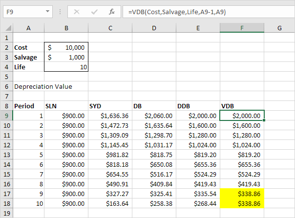 604×447 depreciation formulas excel complete tutorial from www.excel-easy.com
  1601×940 double declining balance simple depreciation guide bench accounting from www.bench.co
 How To Calculate Depreciation Using Double Declining Balance In Excel was posted in October 27, 2025 at 6:42 pm. If you wanna have it as yours, please click the Pictures and you will go to click right mouse then Save Image As and Click Save and download the How To Calculate Depreciation Using Double Declining Balance In Excel Picture.. Don’t forget to share this picture with others via Facebook, Twitter, Pinterest or other social medias! we do hope you'll get inspired by ExcelKayra... Thanks again! If you have any DMCA issues on this post, please contact us!