Home » Excel Templates » How To Calculate Weighted Grade Average In Excel

How To Calculate Weighted Grade Average In Excel

Wednesday, June 18th 2025. | Excel Templates

How To Calculate Weighted Grade Average In Excel - There are a lot of affordable templates out there, but it can be easy to feel like a lot of the best cost a amount of money, require best special design template. Making the best template format choice is way to your template success. And if at this time you are looking for information and ideas regarding the How To Calculate Weighted Grade Average In Excel then, you are in the perfect place. Get this How To Calculate Weighted Grade Average In Excel for free here. We hope this post How To Calculate Weighted Grade Average In Excel inspired you and help you what you are looking for.

weighted average excel step step tutorial

“`html

Calculating Weighted Grade Average in Excel

Calculating your grade point average (GPA) when different assignments or exams carry different weights can be tricky. Luckily, Microsoft Excel provides a powerful and relatively simple way to calculate a weighted average. This guide will walk you through the process step-by-step, covering the common scenarios and providing tips for making your spreadsheet more organized and user-friendly.

Understanding Weighted Averages

Before diving into Excel, let’s quickly review the concept of a weighted average. A weighted average considers the importance (weight) of each individual value in a dataset. Unlike a simple average where all values are treated equally, a weighted average assigns more influence to values with higher weights. In the context of grades, an exam worth 50% of your final grade will have a much larger impact than a quiz worth only 5%.

The formula for a weighted average is as follows:

Weighted Average = (Value 1 * Weight 1) + (Value 2 * Weight 2) + … + (Value n * Weight n) / (Weight 1 + Weight 2 + … + Weight n)

Where:

Value represents the individual grade or score.
Weight represents the proportion or percentage that the grade contributes to the overall grade.

Setting Up Your Excel Spreadsheet

First, create a new Excel spreadsheet. You’ll need columns for the assignment names, the grades received, and the weights assigned to each assignment. A suggested layout looks like this:

Column A: Assignment Name (e.g., “Midterm Exam,” “Homework 1,” “Final Project”)
Column B: Grade Received (e.g., 85, 92, 78)
Column C: Weight (e.g., 0.25, 0.10, 0.40). Weights should be expressed as decimals (percentages divided by 100).

Fill in your spreadsheet with the appropriate data. For example:

Assignment Name	Grade Received	Weight
Midterm Exam	85	0.25
Homework 1	92	0.10
Homework 2	88	0.10
Final Project	78	0.40
Participation	95	0.15

Calculating the Weighted Average

Now, let’s calculate the weighted average using Excel formulas.

Calculate the Weighted Score for Each Assignment: In a new column (e.g., Column D), you’ll multiply the Grade Received (Column B) by the Weight (Column C) for each assignment. In cell D2, enter the following formula: =B2*C2. Then, drag the fill handle (the small square at the bottom right of the cell) down to apply this formula to all the rows containing your assignments. This will calculate the weighted score for each item.
Calculate the Sum of the Weighted Scores: In a new cell (e.g., D7), use the SUM function to add up all the weighted scores you just calculated in Column D. Enter the following formula: =SUM(D2:D6) (adjust the range D2:D6 to match the actual range of your weighted scores).
Calculate the Sum of the Weights: It’s crucial to ensure that the weights add up to 1 (or 100%). In another cell (e.g., C7), use the SUM function to add up all the weights in Column C. Enter the following formula: =SUM(C2:C6) (again, adjust the range to match your data). This step helps you verify the accuracy of your weights and identify potential errors.
Calculate the Weighted Average: Finally, divide the sum of the weighted scores (calculated in step 2) by the sum of the weights (calculated in step 3). In a new cell (e.g., E7), enter the following formula: =D7/C7. This cell will now display your weighted grade average.

Using the SUMPRODUCT Function (A More Efficient Method)

Excel offers a more concise way to calculate the weighted average using the SUMPRODUCT function. This function multiplies corresponding components in given arrays and returns the sum of those products.

Enter the SUMPRODUCT Formula: In a new cell (e.g., E8), enter the following formula: =SUMPRODUCT(B2:B6,C2:C6)/SUM(C2:C6).

Here’s how this formula works:

SUMPRODUCT(B2:B6,C2:C6): This part multiplies each grade in the range B2:B6 by its corresponding weight in the range C2:C6 and then sums up those products. This effectively performs the calculation: (B2*C2) + (B3*C3) + (B4*C4) + (B5*C5) + (B6*C6).
SUM(C2:C6): This part calculates the sum of all the weights, ensuring that the weighted average is correctly normalized (divided by the total weight).
/: The division operator divides the sum of the products by the sum of the weights, giving you the final weighted average.

The result in cell E8 should be the same as the result you obtained using the step-by-step method. The SUMPRODUCT function is generally preferred for its conciseness and efficiency.

Verifying Your Weights

It is absolutely critical to verify that your weights sum to 1 (or 100%). If the sum of the weights is not equal to 1, your weighted average calculation will be incorrect. Excel can help you easily identify this problem.

Conditional Formatting: Use conditional formatting to highlight the cell containing the sum of the weights if it is not equal to 1. Select the cell (e.g., C7) containing the sum of the weights. Go to Home > Conditional Formatting > New Rule… Choose “Use a formula to determine which cells to format.” In the formula box, enter =C7<>1 (replace C7 with the actual cell containing the sum of the weights). Click the “Format…” button and choose a fill color (e.g., red) to highlight the cell if the formula is true (i.e., the sum of the weights is not equal to 1). Click OK to save the rule. Now, if the sum of the weights is anything other than 1, the cell will be highlighted, alerting you to the error.

Adding Formatting and Labels

To make your spreadsheet more readable and professional, consider adding the following formatting elements:

Headers: Bold the column headers (Assignment Name, Grade Received, Weight, Weighted Score).
Number Formatting: Format the “Grade Received” column as a number with no decimal places. Format the “Weight” column as a percentage with two decimal places (e.g., 25.00%). Format the weighted average cell as a number with two decimal places.
Labels: Add labels to the cells containing the sum of the weights and the weighted average (e.g., “Total Weight:” and “Weighted Average:”).
Borders: Add borders to the table for better visual separation.
Color Coding: Use different background colors for headers, data rows, and summary cells to improve clarity.

Example with Letter Grades

If your grades are in letter format (A, B, C, etc.), you’ll first need to convert them to numerical values before calculating the weighted average. You can use a lookup table or nested IF statements to achieve this.

Create a Lookup Table: In a separate part of your spreadsheet, create a table that maps letter grades to numerical values (e.g., A=4.0, B=3.0, C=2.0, D=1.0, F=0.0).
Use the VLOOKUP Function: In the “Grade Received” column, use the VLOOKUP function to look up the numerical equivalent of each letter grade from your lookup table. For example, if your letter grades are in Column B and your lookup table is in the range F1:G5, the formula in Column C would be: =VLOOKUP(B2,F1:G5,2,FALSE). This formula looks up the letter grade in cell B2 in the first column of the lookup table (F1:F5), and returns the corresponding numerical value from the second column (G1:G5). The `FALSE` argument ensures an exact match.
Proceed with Weighted Average Calculation: Once you have the numerical equivalents of the letter grades, you can proceed with the weighted average calculation as described earlier.

Troubleshooting

Incorrect Weights: Double-check that all weights are entered correctly and that they sum to 1 (or 100%). Use conditional formatting to highlight errors.
Formula Errors: Carefully review your formulas for typos or incorrect cell references. Use Excel’s formula auditing tools to help identify errors.
Circular References: Avoid creating circular references, where a formula refers to its own cell, directly or indirectly. This can lead to incorrect results.
Division by Zero: Ensure that the cell containing the sum of the weights is not zero. If it is, you’ll get a #DIV/0! error.

By following these steps and using Excel’s powerful features, you can easily and accurately calculate your weighted grade average, giving you a clear understanding of your academic performance.

“`

700×400 excel formula weighted average exceljet from exceljet.net

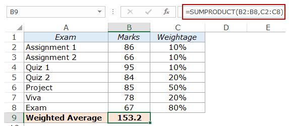573×250 calculating weighted average excel formulas from trumpexcel.com

410×363 calculate weighted average excel fast easy from spreadsheeto.com

1024×576 calculate weighted average excel easyclick from www.easyclickacademy.com

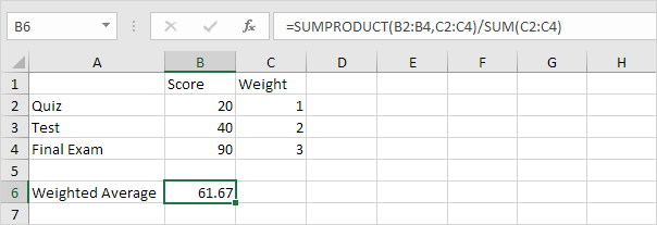604×207 weighted average excel step step tutorial from www.excel-easy.com

534×340 weighted average excel calculate weighted average excel from www.educba.com

648×449 finding weighted average excel deskbright from www.deskbright.com

849×283 weighted average calculations excel student percentage marks from www.bluepecantraining.com

How To Calculate Weighted Grade Average In Excel was posted in June 18, 2025 at 6:10 am. If you wanna have it as yours, please click the Pictures and you will go to click right mouse then Save Image As and Click Save and download the How To Calculate Weighted Grade Average In Excel Picture.. Don’t forget to share this picture with others via Facebook, Twitter, Pinterest or other social medias! we do hope you'll get inspired by ExcelKayra... Thanks again! If you have any DMCA issues on this post, please contact us!