How To Create A Dynamic Dropdown List In Excel
How To Create A Dynamic Dropdown List In Excel - There are a lot of affordable templates out there, but it can be easy to feel like a lot of the best cost a amount of money, require best special design template. Making the best template format choice is way to your template success. And if at this time you are looking for information and ideas regarding the How To Create A Dynamic Dropdown List In Excel then, you are in the perfect place. Get this How To Create A Dynamic Dropdown List In Excel for free here. We hope this post How To Create A Dynamic Dropdown List In Excel inspired you and help you what you are looking for.
Creating Dynamic Dropdown Lists in Excel
Dynamic dropdown lists in Excel provide a powerful way to create interactive and user-friendly spreadsheets. Unlike static dropdowns where the list of options is fixed, dynamic dropdowns automatically update based on changes in the source data. This makes your spreadsheets more adaptable, less prone to errors, and easier to maintain. This document will guide you through different methods of creating dynamic dropdown lists in Excel.
Method 1: Using Named Ranges with OFFSET Function
This is a classic and widely used method. It relies on defining a named range that dynamically adjusts its size based on the number of valid entries in your data source.
Step 1: Prepare Your Data Source
First, you need a column of data that will serve as the source for your dropdown list. Ensure that this data is in a contiguous range, ideally without any blank cells in the middle of the data.
Example:
Suppose you have a list of fruits in column A, starting from cell A2:
| Column A (Fruits) |
|---|
| Apple |
| Banana |
| Orange |
| Grapes |
| Mango |
Step 2: Create a Named Range with OFFSET
- Go to the “Formulas” tab on the Excel ribbon.
- Click on “Define Name” in the “Defined Names” group.
- In the “New Name” dialog box:
- Name: Enter a name for your range. Let’s call it “FruitList”.
- Scope: Leave it as “Workbook” unless you need it restricted to a specific sheet.
- Refers to: Enter the following formula:
=OFFSET(Sheet1!$A$2,0,0,COUNTA(Sheet1!$A:$A)-1,1)Explanation of the Formula:
OFFSET(reference, rows, cols, height, width)is the core function.Sheet1!$A$2is the starting cell of your data range. Modify this to match your sheet name and starting cell.0, 0means we’re not offsetting the starting cell by any rows or columns.COUNTA(Sheet1!$A:$A)-1calculates the number of non-blank cells in column A (including the header) and subtracts 1 to exclude the header itself. This determines the height (number of rows) of your dynamic range. Modify `Sheet1!$A:$A` to match your source column.1sets the width of the range to 1 column.
- Click “OK”.
Step 3: Create the Dropdown List
- Select the cell where you want the dropdown list to appear.
- Go to the “Data” tab on the Excel ribbon.
- Click on “Data Validation” in the “Data Tools” group.
- In the “Data Validation” dialog box:
- In the “Settings” tab:
- Allow: Choose “List”.
- Source: Enter
=FruitList(or whatever you named your range). - Ignore blank: Check this box to prevent blank entries in the dropdown.
- In-cell dropdown: Check this box to display the dropdown arrow.
- (Optional) Configure the “Input Message” and “Error Alert” tabs for user guidance and error handling.
- In the “Settings” tab:
- Click “OK”.
Now, when you add or remove items from your fruit list in column A, the dropdown list will automatically update.
Method 2: Using Excel Tables
Excel Tables are a structured way to manage data and offer built-in dynamic resizing. This makes them ideal for creating dynamic dropdowns.
Step 1: Create an Excel Table
- Select your data range (including the header).
- Go to the “Insert” tab on the Excel ribbon.
- Click on “Table” in the “Tables” group.
- In the “Create Table” dialog box:
- Make sure “My table has headers” is checked if your data includes a header row.
- Click “OK”.
Your data is now formatted as an Excel Table. Note the default table name (e.g., Table1) which can be changed in the “Table Design” tab (which appears when the table is selected) under the “Properties” group.
Step 2: Define a Named Range Referring to the Table Column
- Go to the “Formulas” tab on the Excel ribbon.
- Click on “Define Name” in the “Defined Names” group.
- In the “New Name” dialog box:
- Name: Enter a name for your range. Let’s call it “FruitListTable”.
- Scope: Leave it as “Workbook”.
- Refers to: Enter the following formula:
=Table1[Fruits]Explanation of the Formula:
Table1is the name of your Excel Table. Replace this if you renamed your table.[Fruits]is the name of the column containing the fruit data within the table. Replace “Fruits” with the actual column header. This uses structured references, a powerful feature of Excel Tables.
- Click “OK”.
Step 3: Create the Dropdown List
Follow the same steps as in Method 1, but in the “Data Validation” dialog box, in the “Source” field, enter =FruitListTable (or whatever you named your range referring to the table column).
Now, when you add or remove rows in the Excel Table, the dropdown list will automatically update because the named range is dynamically linked to the table.
Method 3: Using Dynamic Arrays (Excel 365 and later)
Excel 365 introduced dynamic arrays, which greatly simplifies creating dynamic lists. The FILTER, UNIQUE, and SORT functions are incredibly useful.
Step 1: Prepare Your Data Source
Same as in previous methods.
Step 2: Create a Dynamic Array Formula
In a separate column (e.g., Column C), enter the following formula, assuming your data starts in A2:
=SORT(UNIQUE(FILTER(A2:A1000, A2:A1000<>"")))
Explanation of the Formula:
FILTER(A2:A1000, A2:A1000<>"")filters the range A2:A1000, returning only the non-blank cells. Adjust A2:A1000 to cover a reasonably large expected data range.UNIQUE(FILTER(...))ensures that only unique values are returned from the filtered range.SORT(UNIQUE(FILTER(...)))sorts the unique values alphabetically.
This single formula will spill the resulting dynamic array down the column. Excel automatically handles the range expansion as new data is added.
Step 3: Create a Named Range
- Go to the “Formulas” tab on the Excel ribbon.
- Click on “Define Name” in the “Defined Names” group.
- In the “New Name” dialog box:
- Name: Enter a name for your range. Let’s call it “FruitListDynamic”.
- Scope: Leave it as “Workbook”.
- Refers to: Enter the following formula, assuming your dynamic array formula is in cell C2:
=Sheet1!$C$2#Explanation of the Formula:
Sheet1!$C$2is the cell containing the dynamic array formula.- The
#symbol is the spill range operator. It tells Excel to refer to the entire spilled array starting from cell C2. This automatically adjusts as the array grows or shrinks.
- Click “OK”.
Step 4: Create the Dropdown List
Follow the same steps as in Method 1, but in the “Data Validation” dialog box, in the “Source” field, enter =FruitListDynamic.
This method is the most elegant and efficient in Excel 365 because the dynamic array automatically handles updates and the spill range operator ensures the dropdown list always reflects the current data.
Tips and Considerations
* **Error Handling:** Implement error handling in your formulas to prevent errors if the data source is empty or contains unexpected values. The `IFERROR` function can be helpful. * **Blank Cells:** Be mindful of blank cells in your data source, as they might appear as blank options in your dropdown list. Use the `FILTER` function (as in Method 3) or the “Ignore blank” option in Data Validation to address this. * **Data Validation Settings:** Explore the “Input Message” and “Error Alert” tabs in the Data Validation dialog box to provide helpful instructions and error messages to users. * **Sorting:** If you want your dropdown list to be sorted alphabetically, use the `SORT` function (as demonstrated in Method 3) within your dynamic range definition. * **Data Type Consistency:** Ensure that the data in your source column is consistent (e.g., all text or all numbers). Inconsistent data types can lead to unexpected behavior. * **Performance:** For very large datasets, using dynamic arrays (Method 3) often provides better performance than OFFSET-based solutions (Method 1). * **Dependencies:** Avoid circular references or complex dependencies that could slow down your spreadsheet. * **Accessibility:** Consider the accessibility of your dropdown lists for users with disabilities. Provide clear labels and instructions.
By mastering these methods, you can create dynamic and user-friendly dropdown lists that significantly enhance the functionality and usability of your Excel spreadsheets. Choose the method that best suits your Excel version and the complexity of your data. Remember to test your dropdown lists thoroughly after implementing them to ensure they are working correctly.
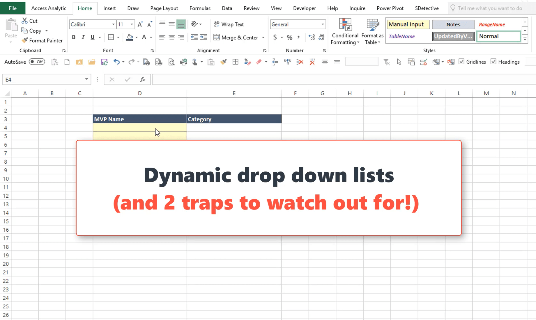 1841×1101 create dynamic drop list excel access analytic from accessanalytic.com.au
  1280×600 dynamic dropdown list excel microsoft office from ms-office.wonderhowto.com
  1334×993 create dynamic drop list excel excel unlocked from excelunlocked.com
  1011×609 create dynamic drop list excel gyankosh learning from gyankosh.net
  605×614 dropdown list excel puresourcecode from www.puresourcecode.com
 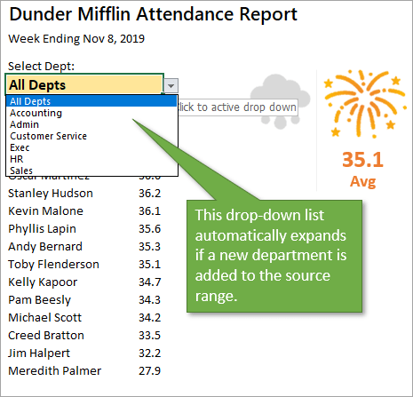 465×447 create dynamic drop list automatically expands from www.excelcampus.com
 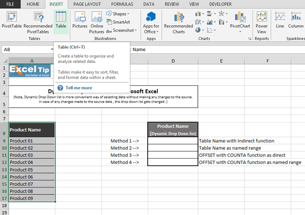 624×439 create dynamic drop list excel methods from www.exceltip.com
 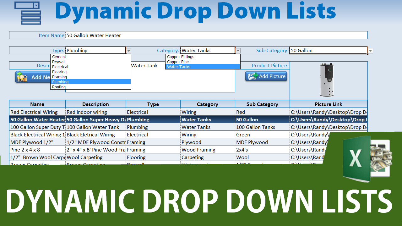 1280×719 excel dynamic drop lists workbook excel from www.excelforfreelancers.com
  821×626 create dynamic drop lists excel stl blog from www.stl-training.co.uk
 How To Create A Dynamic Dropdown List In Excel was posted in February 24, 2026 at 2:29 pm. If you wanna have it as yours, please click the Pictures and you will go to click right mouse then Save Image As and Click Save and download the How To Create A Dynamic Dropdown List In Excel Picture.. Don’t forget to share this picture with others via Facebook, Twitter, Pinterest or other social medias! we do hope you'll get inspired by ExcelKayra... Thanks again! If you have any DMCA issues on this post, please contact us!