How To Create Cascading Dropdown Lists In Excel
How To Create Cascading Dropdown Lists In Excel - There are a lot of affordable templates out there, but it can be easy to feel like a lot of the best cost a amount of money, require best special design template. Making the best template format choice is way to your template success. And if at this time you are looking for information and ideas regarding the How To Create Cascading Dropdown Lists In Excel then, you are in the perfect place. Get this How To Create Cascading Dropdown Lists In Excel for free here. We hope this post How To Create Cascading Dropdown Lists In Excel inspired you and help you what you are looking for.
“`html
Creating Cascading Dropdown Lists in Excel
Cascading dropdown lists, also known as dependent dropdown lists, are a powerful feature in Excel that allows you to create a series of related dropdown menus. Selecting an option in one dropdown will filter the available choices in subsequent dropdowns, creating a more user-friendly and efficient data entry experience. Imagine selecting a country in the first dropdown, and then the second dropdown automatically populates with only the cities within that country. This is the power of cascading dropdowns.
Understanding the Concept
The core principle behind cascading dropdowns involves using Excel’s data validation feature in conjunction with formulas like INDEX, MATCH, and OFFSET (or FILTER in newer versions of Excel). We define named ranges corresponding to the possible choices in each dropdown level. The selection in the first dropdown determines which named range is used as the source for the second dropdown, and so on.
Step-by-Step Guide
Let’s create a simple example of cascading dropdowns for **Category**, **Subcategory**, and **Item**. Assume we have the following data:
- **Category:** Electronics, Clothing, Food
- **Electronics Subcategories:** Laptops, Smartphones, Headphones
- **Clothing Subcategories:** Shirts, Pants, Shoes
- **Food Subcategories:** Fruits, Vegetables, Dairy
- **Laptops Items:** Dell, HP, Apple
- **Smartphones Items:** Samsung, Google, Apple
- **Headphones Items:** Sony, Bose, Jabra
- **Shirts Items:** Polo, T-Shirt, Button-Down
- **Pants Items:** Jeans, Shorts, Dress Pants
- **Shoes Items:** Sneakers, Sandals, Boots
- **Fruits Items:** Apples, Bananas, Oranges
- **Vegetables Items:** Carrots, Broccoli, Spinach
- **Dairy Items:** Milk, Cheese, Yogurt
1. Prepare Your Data
Organize your data in a clear, structured format on a separate sheet (e.g., Sheet2). This sheet will act as your data source for the dropdown lists. It’s best to structure your data horizontally. For example:
| Category | Electronics | Clothing | Food |
|---|---|---|---|
| Subcategory | Laptops | Shirts | Fruits |
| Smartphones | Pants | Vegetables | |
| Headphones | Shoes | Dairy |
| Subcategory | Laptops | Smartphones | Headphones | Shirts | Pants | Shoes | Fruits | Vegetables | Dairy |
|---|---|---|---|---|---|---|---|---|---|
| Item | Dell | Samsung | Sony | Polo | Jeans | Sneakers | Apples | Carrots | Milk |
| HP | Bose | T-Shirt | Shorts | Sandals | Bananas | Broccoli | Cheese | ||
| Apple | Apple | Jabra | Button-Down | Dress Pants | Boots | Oranges | Spinach | Yogurt |
2. Define Named Ranges
Now, define named ranges for each category and its associated subcategories and items. This is crucial for the data validation formulas to work correctly.
- **Category:** Select the cells containing the categories (e.g., B1:D1 in the first table). Go to the “Formulas” tab and click “Define Name”. Enter “CategoryList” (or any name you prefer, but be consistent) in the “Name” field and click “OK”.
- **Electronics, Clothing, Food:** For each category, create a named range for its corresponding subcategories. Select the cells containing the subcategories for “Electronics” (e.g., B2:B4 in the first table). Define a name as “ElectronicsList”. Repeat this for “Clothing” (C2:C4 -> “ClothingList”) and “Food” (D2:D4 -> “FoodList”).
- **Subcategories -> Items:** Repeat the process for each Subcategory in the second table. For example, select the items for “Laptops” (B2:B4 -> “LaptopsList”), “Smartphones” (C2:C4 -> “SmartphonesList”), and so on. Ensure that each named range corresponds to the correct subcategory.
Important: The names of the subcategory lists (ElectronicsList, ClothingList, FoodList) *must* match the *exact* values in the CategoryList. This is how Excel knows which list to display.
3. Create the Dropdown Lists on Your Main Sheet
Now, switch to the sheet where you want to create the cascading dropdowns (e.g., Sheet1).
- **Category Dropdown:** Select the cell where you want the “Category” dropdown (e.g., A1). Go to the “Data” tab and click “Data Validation”. In the “Settings” tab:
- Allow: List
- Source: =CategoryList (enter the name you assigned to the category list)
- Click “OK”.
- **Subcategory Dropdown:** Select the cell where you want the “Subcategory” dropdown (e.g., B1). Go to “Data Validation” and in the “Settings” tab:
- Allow: List
- Source: =INDIRECT(A1&”List”) (replace A1 with the cell containing the Category dropdown)
- Click “OK”.
- **Item Dropdown:** Select the cell where you want the “Item” dropdown (e.g., C1). Go to “Data Validation” and in the “Settings” tab:
- Allow: List
- Source: =INDIRECT(B1&”List”) (replace B1 with the cell containing the Subcategory dropdown)
- Click “OK”.
Explanation of INDIRECT function:
The INDIRECT function is the key to making this work. It takes a text string as an argument and returns the reference specified by that string. For example, if cell A1 contains the text “Electronics”, then INDIRECT(A1&"List") will evaluate to INDIRECT("ElectronicsList"), which then resolves to the named range “ElectronicsList”. This is why the named ranges *must* match the values in the preceding dropdown, with “List” appended.
4. Testing Your Cascading Dropdowns
Now, test your dropdowns. Select a category from the first dropdown. The second dropdown should populate with only the subcategories associated with that category. Selecting a subcategory will, in turn, populate the item dropdown with relevant items.
Alternative using the FILTER function (Excel 365 and later)
Newer versions of Excel provide the FILTER function, which can simplify the creation of cascading dropdowns. This method avoids the need for separate named ranges for each subcategory/item.
Data Preparation:
Instead of the previous horizontal layout, structure your data vertically like this:
| Category | Subcategory | Item |
|---|---|---|
| Electronics | Laptops | Dell |
| Electronics | Laptops | HP |
| Electronics | Laptops | Apple |
| Electronics | Smartphones | Samsung |
| Electronics | Smartphones | |
| Electronics | Smartphones | Apple |
Named Ranges (using FILTER):
- **Category:** Define the named range “CategoryList” as before, pointing to the unique list of categories (e.g., =UNIQUE(Sheet2!A:A)). The
UNIQUEfunction ensures only distinct categories are included. - **SubcategoryFilterRange:** Select the entire data table including headers (A1:C[last row]) on Sheet2 and define the named range as “DataTable”.
- **ItemFilterRange:** Same as “SubcategoryFilterRange”
Dropdown Creation (using FILTER):
- **Category Dropdown:** Select the cell where you want the “Category” dropdown (e.g., A1). Go to the “Data” tab and click “Data Validation”. In the “Settings” tab:
- Allow: List
- Source: =CategoryList (enter the name you assigned to the category list)
- Click “OK”.
- **Subcategory Dropdown:** Select the cell where you want the “Subcategory” dropdown (e.g., B1). Go to “Data Validation” and in the “Settings” tab:
- Allow: List
- Source: =UNIQUE(FILTER(DataTable[Subcategory],DataTable[Category]=A1,””))
- Click “OK”.
- **Item Dropdown:** Select the cell where you want the “Item” dropdown (e.g., C1). Go to “Data Validation” and in the “Settings” tab:
- Allow: List
- Source: =UNIQUE(FILTER(DataTable[Item],DataTable[Subcategory]=B1,””))
- Click “OK”.
Explanation of FILTER formula:
=UNIQUE(FILTER(DataTable[Subcategory],DataTable[Category]=A1,"")):
FILTER(DataTable[Subcategory],DataTable[Category]=A1,"")filters the “Subcategory” column from the “DataTable” where the corresponding “Category” equals the value in cell A1 (the selected category). If no match is found, it returns an empty string (“”).UNIQUE(...)returns a unique list of the filtered subcategories, preventing duplicates from appearing in the dropdown.
Troubleshooting
- Dropdowns are blank: Double-check that your named ranges are defined correctly and that they point to the correct data. Verify that the
INDIRECTformulas are referencing the correct cells. For the FILTER function make sure the ranges are pointing to the correct columns. - Error messages: If you get an error message like “#REF!”, it usually means that the
INDIRECTfunction is trying to reference a non-existent named range. Ensure the spelling of your named ranges is consistent and matches the values in the preceding dropdown (with “List” appended). - Dropdowns don’t update: Make sure automatic calculation is enabled in Excel (Formulas tab -> Calculation Options -> Automatic).
Conclusion
Cascading dropdown lists enhance your Excel spreadsheets by providing a dynamic and user-friendly way to input data. By using named ranges and either INDIRECT or the FILTER function, you can create a powerful and intuitive data entry experience. Choose the method that best suits your Excel version and data structure. Remember to carefully plan your data layout and consistently name your ranges for optimal results.
“`
 306×182 dependent cascading drop list excel ablebitscom from www.ablebits.com
 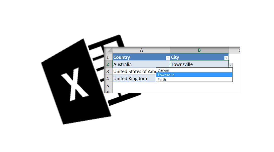 1050×581 excel cascading drop vba analyst cave from analystcave.com
  901×303 create dynamic cascading list boxes excel kamil from kamiltech.com
 How To Create Cascading Dropdown Lists In Excel was posted in October 26, 2025 at 7:14 am. If you wanna have it as yours, please click the Pictures and you will go to click right mouse then Save Image As and Click Save and download the How To Create Cascading Dropdown Lists In Excel Picture.. Don’t forget to share this picture with others via Facebook, Twitter, Pinterest or other social medias! we do hope you'll get inspired by ExcelKayra... Thanks again! If you have any DMCA issues on this post, please contact us!