Home » Excel Templates » How To Create Drop Down List In Excel With Data Validation

How To Create Drop Down List In Excel With Data Validation

Thursday, December 25th 2025. | Excel Templates

How To Create Drop Down List In Excel With Data Validation - There are a lot of affordable templates out there, but it can be easy to feel like a lot of the best cost a amount of money, require best special design template. Making the best template format choice is way to your template success. And if at this time you are looking for information and ideas regarding the How To Create Drop Down List In Excel With Data Validation then, you are in the perfect place. Get this How To Create Drop Down List In Excel With Data Validation for free here. We hope this post How To Create Drop Down List In Excel With Data Validation inspired you and help you what you are looking for.

understanding excel data validation rockets marketing

“`html

Creating Drop-Down Lists in Excel with Data Validation

Drop-down lists in Excel offer a powerful way to control data entry, ensure consistency, and simplify spreadsheet usage. They constrain users to select from a predefined set of options, reducing errors and making data analysis more reliable. Excel’s data validation feature makes creating these drop-down lists straightforward. This guide will walk you through the process step-by-step, covering various scenarios and advanced techniques.

Basic Drop-Down List Creation

The simplest method involves directly specifying the list of allowed values within the data validation settings.

Select the Cell(s): Begin by selecting the cell or range of cells where you want the drop-down list to appear.
Access Data Validation: Navigate to the “Data” tab on the Excel ribbon. Click on “Data Validation” in the “Data Tools” group. This opens the Data Validation dialog box.
Choose “List” as the Validation Criteria: In the “Settings” tab of the Data Validation dialog box, under “Allow,” select “List” from the drop-down menu.
Enter the Source List: In the “Source” box, type the items you want to appear in the drop-down list, separated by commas. For example: Yes,No,Maybe. Ensure there are no extra spaces before or after the commas.
Configure Error Alert (Optional): The “Error Alert” tab allows you to customize what happens when a user enters a value that isn’t in the list. You can choose a style (Stop, Warning, or Information), a title, and an error message. A “Stop” style prevents the user from entering invalid data. “Warning” and “Information” styles allow the user to proceed but display a message.
Configure Input Message (Optional): The “Input Message” tab allows you to display a message to the user when they select a cell with the drop-down list. This message can provide instructions or context. You can specify a title and an input message.
Click “OK”: Click “OK” to apply the data validation settings. The selected cells will now have a drop-down arrow, and clicking it will reveal your list of options.

Using a Cell Range as the Source List

This method is ideal when your list is long or when you want to easily update the list without modifying the data validation settings directly. It involves referencing a range of cells containing the allowed values.

Prepare the List: Create a list of allowed values in a column or row in your spreadsheet. This list can be on the same sheet or a different sheet. Ensure the list is contiguous (no blank cells in between the values).
Select the Cell(s): Select the cell or range of cells where you want the drop-down list.
Access Data Validation: Navigate to the “Data” tab and click “Data Validation.”
Choose “List” as the Validation Criteria: In the “Settings” tab, select “List” from the “Allow” drop-down.
Enter the Source Range: In the “Source” box, click the “Sheet” containing your list and then select the range of cells containing the list. You can also type the range directly, for example: Sheet2!A1:A10. Using absolute references (e.g., $A$1:$A$10) prevents the range from changing if you copy the data validation to other cells. If your list is on the same sheet, you can simply type A1:A10.
Configure Error Alert and Input Message (Optional): Customize the “Error Alert” and “Input Message” tabs as needed.
Click “OK”: Click “OK” to create the drop-down list.

Dynamic Drop-Down Lists (Using Named Ranges and OFFSET)

A dynamic drop-down list automatically adjusts its contents when items are added or removed from the source list. This is achieved using named ranges and the OFFSET function.

Create the Source List: Create your list of allowed values. Leave some empty rows below the last item in the list to accommodate future additions.
Define a Named Range:
- Select the entire list of values, *including* the empty rows below the last item.
- Go to the “Formulas” tab and click “Define Name” in the “Defined Names” group. Alternatively, you can type a name in the name box to the left of the formula bar.
- In the “Name” box, enter a descriptive name for your list (e.g., “MyList”).
- In the “Refers to” box, enter the following formula, replacing A1 with the *first cell* in your list of values and `10` with an estimate of the maximum number of items your list will grow to: =OFFSET(Sheet1!$A$1,0,0,COUNTA(Sheet1!$A:$A),1) where Sheet1 is the name of the sheet containing the list.
- Make sure you are using absolute cell references (e.g., `$A$1`).
- Click “OK”.
Create the Drop-Down List:
- Select the cell or range of cells for the drop-down list.
- Go to “Data” > “Data Validation.”
- In the “Settings” tab, select “List.”
- In the “Source” box, type =MyList (or whatever name you assigned to the named range).
- Click “OK.”
Test the Dynamic List: Add or remove items from your source list. The drop-down list will automatically update to reflect the changes.

Tips and Considerations

Blank Cells: If your source list contains blank cells, these will appear as blank options in the drop-down list. To avoid this, ensure your list is contiguous.
Hidden Sheets: You can place your source list on a hidden sheet to keep your spreadsheet cleaner. The data validation will still work correctly.
Error Handling: Carefully configure the “Error Alert” to provide helpful messages to users who enter invalid data. A clear and informative error message can prevent frustration and ensure data quality.
Copying and Pasting: When copying and pasting cells with data validation, be aware of how the validation rules are affected. Use “Paste Special” to control whether the validation rules are copied along with the cell contents.
Data Validation and Formulas: Data validation can be combined with formulas to create more sophisticated data entry controls. For example, you can use a formula in the “Source” box to dynamically generate the list of allowed values based on other cell values.
Using Tables: Converting your source list to an Excel Table simplifies dynamic updates and makes your formulas more readable. Tables automatically expand when you add new rows, and you can refer to table columns by name in your formulas.

By mastering these techniques, you can effectively use drop-down lists in Excel to improve data quality, streamline data entry, and enhance the overall usability of your spreadsheets.

“`

397×312 data validation data validation excel excel drop list excel from myexceltemplates.com

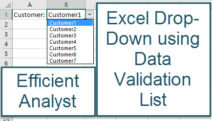434×249 creating excel drop list data validation list efficient from efficientanalyst.com

640×477 create drop lists data validation microsoft excel from www.groovypost.com

950×472 create data validation drop list excel chris menard chris from chrismenardtraining.com

660×440 create drop list excel data validation shortcuts from gaylelarson.com

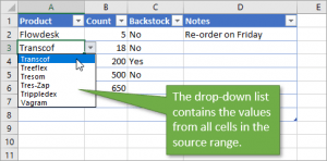300×148 create drop lists excel complete guide video tutorial from www.excelcampus.com

1333×1000 understanding excel data validation rockets marketing from 500rockets.io

3200×2400 create drop list excel pictures wikihow from www.wikihow.com

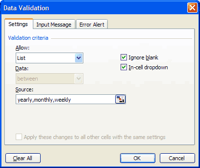408×342 create drop list excel from www.vertex42.com

How To Create Drop Down List In Excel With Data Validation was posted in December 25, 2025 at 11:16 am. If you wanna have it as yours, please click the Pictures and you will go to click right mouse then Save Image As and Click Save and download the How To Create Drop Down List In Excel With Data Validation Picture.. Don’t forget to share this picture with others via Facebook, Twitter, Pinterest or other social medias! we do hope you'll get inspired by ExcelKayra... Thanks again! If you have any DMCA issues on this post, please contact us!