How To Create Interactive Excel Charts Using Slicers And Filters
How To Create Interactive Excel Charts Using Slicers And Filters - There are a lot of affordable templates out there, but it can be easy to feel like a lot of the best cost a amount of money, require best special design template. Making the best template format choice is way to your template success. And if at this time you are looking for information and ideas regarding the How To Create Interactive Excel Charts Using Slicers And Filters then, you are in the perfect place. Get this How To Create Interactive Excel Charts Using Slicers And Filters for free here. We hope this post How To Create Interactive Excel Charts Using Slicers And Filters inspired you and help you what you are looking for.
“`html
Creating Interactive Excel Charts with Slicers and Filters
Excel charts are powerful tools for visualizing data. However, static charts can sometimes fall short in conveying insights effectively. By incorporating slicers and filters, you can transform your charts into interactive dashboards, allowing users to explore data dynamically and uncover hidden patterns.
Understanding Slicers and Filters
Before diving into the how-to, let’s understand the core concepts:
- Slicers: Slicers are visual filters that provide buttons for quickly filtering data in a PivotTable or data range. They offer an intuitive way to select specific items and instantly update the associated chart. Think of them as visual checkpoints, allowing you to narrow down the data displayed based on specific categories.
- Filters: Excel’s filter feature, accessible through the Data tab, allows you to selectively display rows in a data range based on specified criteria. While not as visually appealing as slicers, filters offer powerful filtering capabilities and can be used to control the data source for your charts.
Step-by-Step Guide: Creating Interactive Charts with Slicers (PivotTable Approach)
This approach leverages PivotTables and PivotCharts, the most common and robust method for building interactive dashboards.
- Prepare Your Data: Ensure your data is organized in a table format with clear headers for each column. This is crucial for creating a PivotTable. Avoid empty rows or columns within your data range.
- Create a PivotTable: Select your data range (including headers). Go to the “Insert” tab and click on “PivotTable”. Choose where you want to place the PivotTable (new worksheet or existing one) and click “OK”.
- Design Your PivotTable: In the PivotTable Fields pane (usually on the right), drag and drop the fields you want to analyze into the appropriate areas:
- Rows: Fields you want to display as rows in the PivotTable. These will often be categories or dimensions.
- Columns: Fields you want to display as columns. Use sparingly, as too many columns can make the table unwieldy.
- Values: Fields you want to aggregate (sum, count, average, etc.). These are typically numerical data.
- Filters: Fields you want to use as filters, but not necessarily display in the table itself. You *can* use the PivotTable’s built-in filter options, but slicers offer a better interactive experience.
For example, if you have sales data with columns like “Product,” “Region,” and “Sales Amount,” you might put “Product” in Rows, “Region” in Columns, and “Sales Amount” in Values (set to Sum).
- Create a PivotChart: With your PivotTable selected, go to the “Insert” tab and choose a chart type (e.g., column, line, pie chart) from the “Charts” group. Excel will automatically create a chart based on your PivotTable.
- Insert Slicers: Select your PivotTable (or PivotChart). Go to the “Analyze” tab (which appears when a PivotTable is selected) and click “Insert Slicer”. A dialog box will appear, listing all the fields in your data source. Check the boxes next to the fields you want to use as slicers and click “OK”.
- Customize Your Slicers:
- Positioning and Formatting: Drag and resize the slicers to arrange them neatly around your chart. You can change their colors and styles using the “Slicer Styles” options on the “Slicer” tab (which appears when a slicer is selected).
- Slicer Settings: Right-click on a slicer and choose “Slicer Settings” to customize its behavior:
- Hide items with no data: This removes options that aren’t present in the currently filtered data.
- Sort options: Sort the slicer buttons alphabetically or by data source order.
- Header settings: Change the header text.
- Multi-Select: By default, you can only select one item at a time in a slicer. To allow multi-selection, click the multi-select button (the icon that looks like a funnel with a plus sign) on the slicer toolbar, or hold down the Ctrl key while clicking multiple items.
- Connect Slicers to Multiple PivotTables/Charts (Optional): If you have multiple PivotTables and charts based on the same data source, you can connect a single slicer to all of them. Right-click on the slicer, select “Report Connections,” and check the boxes next to the PivotTables you want to control with that slicer.
- Fine-Tune Your Chart: Customize your chart further by:
- Adding titles and axis labels: Make sure your chart is clearly understandable.
- Adjusting colors and formatting: Use consistent and visually appealing formatting.
- Adding data labels: Display data values directly on the chart elements.
- Changing the chart type: Experiment with different chart types to find the best way to visualize your data.
Using Filters Directly on Data (Non-PivotTable Approach)
While PivotTables offer superior interactivity, you can also use filters directly on your data table to create interactive charts. This approach is suitable for simpler scenarios where you don’t need the aggregation and summarization capabilities of a PivotTable.
- Prepare Your Data: As before, ensure your data is organized in a table format with clear headers.
- Apply Filters: Select your data range (including headers). Go to the “Data” tab and click on “Filter”. Small dropdown arrows will appear in each column header.
- Create Your Chart: Select the data you want to chart (including the headers). Go to the “Insert” tab and choose a chart type.
- Filter Your Data: Use the dropdown arrows in the column headers to filter the data. You can filter by:
- Text Filters: Equals, Contains, Begins With, Ends With, Custom Filter.
- Number Filters: Equals, Greater Than, Less Than, Between, Top 10, Above Average, Below Average, Custom Filter.
- Date Filters: Equals, Before, After, Between, Today, Yesterday, This Week, Last Week, This Month, Last Month, etc.
- Selecting specific items: Uncheck the boxes next to the items you want to exclude from the chart.
Limitations of Direct Filtering: This method directly alters the underlying data visible to the chart. Slicers are often preferred with PivotTables because they don’t modify the original data source, providing a more consistent analysis environment.
Tips for Creating Effective Interactive Charts
- Keep it Simple: Avoid overwhelming users with too many slicers or filters. Choose the most relevant ones for your analysis.
- Clear Labels: Use clear and descriptive labels for slicer buttons and chart elements.
- Consistent Formatting: Use consistent formatting throughout your dashboard to create a professional and polished look.
- Consider Your Audience: Design your dashboard with your target audience in mind. What information are they most interested in? What level of detail do they need?
- Test and Iterate: Test your dashboard with real users to get feedback and make improvements.
- Optimize for Performance: Large datasets and complex PivotTables can impact performance. Optimize your data and PivotTable design to ensure responsiveness. Consider using Excel’s data model for very large datasets.
Conclusion
By mastering the use of slicers and filters, you can transform your Excel charts into dynamic and engaging tools for data exploration. Whether you choose the PivotTable approach for its power and flexibility or direct filtering for simpler scenarios, interactive charts empower users to uncover insights and make data-driven decisions more effectively.
“`
 658×406 excel create interactive charts excel tips mrexcel publishing from www.mrexcel.com
  474×314 create dynamic interactive charts excel from www.extendoffice.com
  477×418 interactive excel charts macros needed from www.contextures.com
  729×768 excel challenge slicers dynamically filter chart excel from www.exceldashboardtemplates.com
 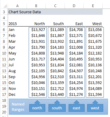 372×397 interactive charts excel visual reference charts chart master from bceweb.org
  557×372 interactive excel charts training hub from www.myonlinetraininghub.com
 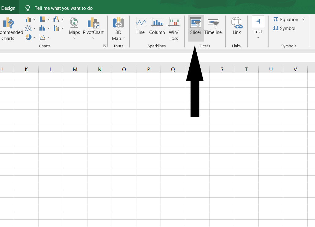 1030×743 create interactive charts excel geeksforgeeks from www.geeksforgeeks.org
  515×319 creating interactive charts slicers simply excel from simplyexcelcoza.weebly.com
 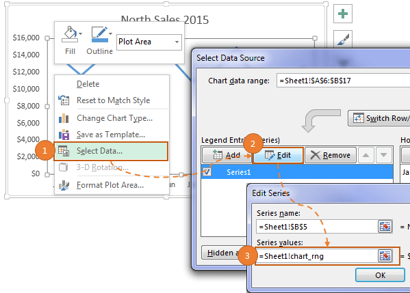 474×339 slicer controlled interactive excel charts from www.myonlinetraininghub.com
  1280×720 interactive excel dashboard tips slicers pi vrogueco from www.vrogue.co
  464×290 charts archives pk excel expert from www.pk-anexcelexpert.com
  932×644 create interactive excel dashboard slicers from maps-for-excel.com
  1280×720 creating interactive excel dashboard slicers pivot charts images from www.tpsearchtool.com
  488×424 slicer formatting demo interactive charts excel pivot table from www.pinterest.com
  640×280 excel slicers introduction tips advanced from www.artofit.org
  600×416 report create type interactive filterslicer excel from superuser.com
  692×268 multiple interactive charts slicers demo interactive charts from www.pinterest.com
  686×532 microsoft excel slicers charts ifonlyidknownthat from ifonlyidknownthat.wordpress.com
  1024×538 chart slicers excel pk excel expert from www.pk-anexcelexpert.com
  528×408 excel slicers introduction tips from www.pinterest.ie
 How To Create Interactive Excel Charts Using Slicers And Filters was posted in March 14, 2026 at 1:51 pm. If you wanna have it as yours, please click the Pictures and you will go to click right mouse then Save Image As and Click Save and download the How To Create Interactive Excel Charts Using Slicers And Filters Picture.. Don’t forget to share this picture with others via Facebook, Twitter, Pinterest or other social medias! we do hope you'll get inspired by ExcelKayra... Thanks again! If you have any DMCA issues on this post, please contact us!