How To Highlight Duplicate Entries Across Sheets In Excel
How To Highlight Duplicate Entries Across Sheets In Excel - There are a lot of affordable templates out there, but it can be easy to feel like a lot of the best cost a amount of money, require best special design template. Making the best template format choice is way to your template success. And if at this time you are looking for information and ideas regarding the How To Highlight Duplicate Entries Across Sheets In Excel then, you are in the perfect place. Get this How To Highlight Duplicate Entries Across Sheets In Excel for free here. We hope this post How To Highlight Duplicate Entries Across Sheets In Excel inspired you and help you what you are looking for.
Highlighting Duplicate Entries Across Sheets in Excel
Identifying duplicate data is a common task in Excel, especially when working with multiple sheets containing similar or related information. This document outlines several methods to highlight duplicate entries across different sheets in Excel, ranging from simple conditional formatting techniques to more advanced solutions using formulas and VBA.
1. Conditional Formatting with a Simple Formula
This method utilizes a basic formula within conditional formatting to check for duplicates across two or more sheets. It’s suitable for smaller datasets where performance isn’t a major concern.
Steps:
- Select the Range: In the first sheet you want to check for duplicates, select the range of cells containing the data you want to analyze (e.g., column A, A1:A100).
- Open Conditional Formatting: Go to the “Home” tab in the Excel ribbon, click on “Conditional Formatting,” then select “New Rule…”
- Choose “Use a formula to determine which cells to format”: In the “New Formatting Rule” dialog box, select this option.
- Enter the Formula: In the formula bar, enter a formula that checks for the existence of the selected cell’s value in another sheet. The formula structure is as follows:
=COUNTIF(Sheet2!$A:$A,A1)>0
ReplaceSheet2with the name of the other sheet you are checking against.$A:$Arepresents the entire column A in Sheet2.A1refers to the first cell in the selected range of the first sheet. It’s crucial to use absolute references ($A:$A) for the range in the other sheet so that it remains constant during the conditional formatting application. The `>0` ensures that the formula returns TRUE only if the value appears at least once in the other sheet. - Set the Formatting: Click the “Format…” button to choose the formatting style you want to apply to the duplicate entries (e.g., fill color, font color, bold).
- Apply the Rule: Click “OK” to close the “Format Cells” dialog box and then click “OK” again to create the conditional formatting rule.
- Repeat for Other Sheets (if necessary): Repeat these steps for other sheets you want to analyze, adjusting the formula to reference the appropriate sheet names.
Explanation:
The COUNTIF function counts the number of times a specific value (A1 in our example) appears within a specified range (Sheet2!$A:$A). If the count is greater than zero, it means the value exists in the other sheet, and the conditional formatting rule applies the selected formatting.
Limitations:
- Performance: This method can be slow for large datasets due to the iterative nature of the
COUNTIFfunction applied to each cell. - Scalability: Managing numerous conditional formatting rules across many sheets can become cumbersome.
- Specific Column: The formula is tailored to check against a specific column (in this case, column A) in the other sheet. If you need to compare against multiple columns, you’ll need to modify the formula.
2. Combining Multiple Columns with CONCATENATE and COUNTIF
If you need to check for duplicates based on multiple columns (e.g., first name and last name), you can combine the values from those columns into a single string using the CONCATENATE function or the & operator, and then use the COUNTIF function to check for duplicates based on this combined string.
Steps:
- Create a Helper Column (if needed): In both sheets, if your duplicate criteria are based on multiple columns, create a helper column that combines the relevant columns. For example, if columns A (first name) and B (last name) are used, in column C, use the formula
=A1&B1or=CONCATENATE(A1,B1)to combine the values. You can add a separator between the names for better readability, such as=A1&"-"&B1. Fill this formula down for all rows in both sheets. If you are checking against a single column, this step is unnecessary. - Select the Range: Select the range containing the combined values (or the single column if you didn’t need a helper) in the first sheet.
- Open Conditional Formatting: Go to the “Home” tab, click “Conditional Formatting,” and select “New Rule…”
- Choose “Use a formula to determine which cells to format”: Select this option in the “New Formatting Rule” dialog.
- Enter the Formula: The formula will now reference the helper column (or the original column if you didn’t create one). For example:
=COUNTIF(Sheet2!$C:$C,C1)>0(if using a helper column in column C)
or
=COUNTIF(Sheet2!$A:$A,A1)>0(if checking only column A).
Remember to replaceSheet2with the actual sheet name. - Set the Formatting: Click “Format…” to choose the formatting style.
- Apply the Rule: Click “OK” to close the dialog boxes.
- Repeat for Other Sheets: Repeat the process for other sheets, adjusting the sheet name in the formula.
Example:
Suppose Sheet1 has “FirstName” in column A and “LastName” in column B, and Sheet2 has the same. In Sheet1, create column C with the formula =A1&B1. In Sheet2, create column C with the formula =A1&B1. Select column C in Sheet1, and apply the conditional formatting rule with the formula =COUNTIF(Sheet2!$C:$C,C1)>0.
3. Using VBA for More Complex Scenarios
For more complex scenarios, such as comparing data across multiple columns and sheets with specific criteria, VBA (Visual Basic for Applications) provides a powerful and flexible solution.
Example VBA Code:
Sub HighlightDuplicatesAcrossSheets() Dim ws1 As Worksheet, ws2 As Worksheet Dim lastRow1 As Long, lastRow2 As Long Dim i As Long, j As Long Dim cell1 As Range, cell2 As Range ' Set the sheet names Set ws1 = ThisWorkbook.Sheets("Sheet1") Set ws2 = ThisWorkbook.Sheets("Sheet2") ' Determine the last row in each sheet lastRow1 = ws1.Cells(Rows.Count, "A").End(xlUp).Row ' Assumes data starts in column A lastRow2 = ws2.Cells(Rows.Count, "A").End(xlUp).Row 'Loop through the data in the first sheet For i = 1 To lastRow1 'Change 1 to the row where your data starts Set cell1 = ws1.Cells(i, "A") 'Set cell1 to the cell in sheet 1, Column A, at the current row 'Loop through the data in the second sheet For j = 1 To lastRow2 'Change 1 to the row where your data starts Set cell2 = ws2.Cells(j, "A") 'Set cell2 to the cell in sheet 2, Column A, at the current row 'Compare the values in both cells If cell1.Value = cell2.Value Then 'If they are equal highlight them in yellow cell1.Interior.Color = vbYellow cell2.Interior.Color = vbYellow End If Next j Next i End Sub
Explanation:
- Declare Variables: The code declares variables to represent the worksheets, last rows, loop counters, and cell ranges.
- Set Worksheet Objects: It assigns the “Sheet1” and “Sheet2” worksheets to the
ws1andws2variables. Important: Change `”Sheet1″` and `”Sheet2″` to the actual names of your sheets. - Determine Last Row: It finds the last row containing data in each sheet using
Cells(Rows.Count, "A").End(xlUp).Row. This assumes data starts in column A. - Nested Loops: It uses nested loops to iterate through each cell in the specified column (“A” in this case) in both sheets. The outer loop iterates through Sheet1, and the inner loop iterates through Sheet2.
- Compare Values: Inside the inner loop, it compares the values of the current cells in both sheets (
cell1.Value = cell2.Value). - Highlight Duplicates: If the values are equal, it highlights both cells in yellow using
cell1.Interior.Color = vbYellowandcell2.Interior.Color = vbYellow. You can change `vbYellow` to any other VBA color constant.
How to Use the VBA Code:
- Open VBA Editor: Press Alt + F11 to open the Visual Basic Editor (VBE).
- Insert a Module: In the VBE, go to “Insert” -> “Module”.
- Paste the Code: Paste the VBA code into the module.
- Modify the Code (if needed):
- Sheet Names: Change
"Sheet1"and"Sheet2"to the actual names of your sheets. - Columns: Change
"A"to the column letter you want to compare. If you need to compare multiple columns, adjust the code to access the relevant column values. - Starting Row: Adjust the loops to start at the correct row containing data (e.g., if your data starts in row 2, change `For i = 1 To lastRow1` to `For i = 2 To lastRow1`).
- Formatting: Change
vbYellowto a different VBA color constant if desired. - Multiple Column Comparison: If you need to compare multiple columns, you will need to adjust the IF statement. For instance, `If cell1.Value = cell2.Value And ws1.Cells(i, “B”).Value = ws2.Cells(j, “B”).Value Then` would check columns A and B for a match.
- Sheet Names: Change
- Run the Code: Go back to Excel and press Alt + F8 to open the “Macro” dialog box. Select the “HighlightDuplicatesAcrossSheets” macro and click “Run”.
Advantages of Using VBA:
- Flexibility: VBA allows you to customize the code to handle complex scenarios, such as comparing multiple columns with specific criteria or applying different formatting based on the type of duplicate.
- Efficiency: VBA can be more efficient than conditional formatting for large datasets, especially when comparing multiple columns or sheets.
- Automation: You can automate the process of highlighting duplicates by creating a button or assigning the macro to a specific event.
Disadvantages of Using VBA:
- Complexity: VBA requires programming knowledge, which may be a barrier for some users.
- Security: Macros can potentially contain malicious code, so it’s important to only run macros from trusted sources. Ensure your macro security settings are appropriate.
Conclusion
Highlighting duplicate entries across sheets in Excel can be achieved using various methods, each with its own advantages and limitations. For simple scenarios involving a single column and small datasets, conditional formatting with a basic formula is a straightforward solution. When dealing with multiple columns or larger datasets, the CONCATENATE and COUNTIF method or VBA provides a more robust and efficient approach. Choose the method that best suits your specific needs and skill level.
 700×400 highlight duplicate values excel formula exceljet from exceljet.net
  700×400 highlight duplicate rows excel formula exceljet from exceljet.net
  914×1030 highlight duplicates multiple worksheets excel formulas from www.exceldemy.com
 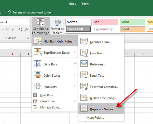 601×487 highlight duplicate entries excel dummytechcom from dummytech.com
  820×508 ways highlight duplicates microsoft excel excel from www.howtoexcel.org
  768×785 excel highlight duplicates sheet from www.statology.org
  513×200 highlight duplicates microsoft excel from www.howtogeek.com
  733×421 highlight duplicates excel examples highlight duplicates from www.educba.com
  1226×538 highlight duplicates excel from www.makeuseof.com
  768×298 epic ways highlight duplicates excel myexcelonline from www.myexcelonline.com
  630×488 find highlight remove duplicates excel from www.exceldemy.com
  492×539 highlight color duplicate entries excel examples from gyankosh.net
  689×436 highlight duplicates excel step step guide from www.wallstreetmojo.com
  1536×836 highlight remove duplicates google sheets from coefficient.io
  1135×815 highlight duplicates excel easy ways guiding tech from www.guidingtech.com
 How To Highlight Duplicate Entries Across Sheets In Excel was posted in February 20, 2026 at 8:44 am. If you wanna have it as yours, please click the Pictures and you will go to click right mouse then Save Image As and Click Save and download the How To Highlight Duplicate Entries Across Sheets In Excel Picture.. Don’t forget to share this picture with others via Facebook, Twitter, Pinterest or other social medias! we do hope you'll get inspired by ExcelKayra... Thanks again! If you have any DMCA issues on this post, please contact us!