Highlighting Duplicate Values Across Multiple Sheets in Excel

Identifying duplicate data is a common task in Excel, especially when working with large datasets spread across multiple worksheets. Highlighting these duplicates allows for easier review, cleaning, and data validation. This guide will walk you through various methods to highlight duplicate values across different sheets in Excel, covering both basic and more advanced techniques.

Understanding the Challenge

Excel’s built-in “Conditional Formatting” feature is excellent for highlighting duplicates within a single sheet. However, directly applying this feature across multiple sheets doesn’t work as expected because it treats each sheet independently. The core challenge is to compare values across these sheets and identify those that exist in more than one.

Method 1: Combining Data into a Single Sheet

The simplest, though potentially resource-intensive for very large datasets, approach is to consolidate all data into a single sheet. This enables you to leverage Excel’s native duplicate highlighting capabilities. Here’s how:

1. Create a Summary Sheet: Insert a new blank sheet. This will be your master sheet for combined data.
2. Copy Data from Each Sheet: Starting with the first sheet containing data, select the range of cells containing the data you want to check for duplicates. Be sure to include the header row for consistency and clarity. Press `Ctrl+C` (or `Cmd+C` on Mac) to copy.
3. Paste into the Summary Sheet: In the summary sheet, click on cell `A1` (or the first cell where you want to paste the data) and press `Ctrl+V` (or `Cmd+V` on Mac) to paste the copied data.
4. Repeat for All Sheets: Repeat steps 2 and 3 for each sheet containing data, pasting each subsequent set of data below the previously pasted data in the summary sheet. Ensure the data columns are aligned correctly.
5. Highlight Duplicates: Now that you have all the data in one sheet:
   • Select the entire data range (including headers) in the summary sheet.
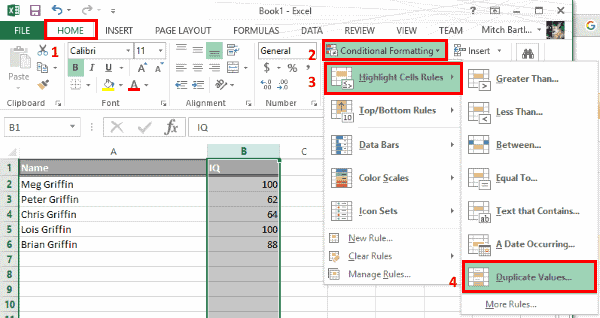
   • Go to the “Home” tab on the Excel ribbon.
   • Click on “Conditional Formatting” in the “Styles” group.
   • Choose “Highlight Cells Rules” and then “Duplicate Values…”.
   • In the “Duplicate Values” dialog box, you can choose the formatting style (e.g., light red fill with dark red text) to highlight the duplicates. Click “OK”.

Pros: Easy to implement, utilizes Excel’s built-in functionality.

Cons: Creates a redundant copy of the data, may be slow with very large datasets, doesn’t automatically update if original data changes.

Method 2: Using the `COUNTIF` Function and Conditional Formatting

This method uses the `COUNTIF` function to count the occurrences of each value across all the sheets and then uses conditional formatting to highlight values that appear more than once. This is a more dynamic approach than the first method.

1. Create a Helper Column: In each sheet where you want to highlight duplicates, add a new column next to the column you’re checking for duplicates (e.g., if you’re checking column A, add a helper column in column B). Label this column appropriately, such as “Duplicate Check”.
2. Use the `COUNTIF` Function: In the first cell of the helper column (e.g., B2 if your data starts in A2), enter the following formula, making adjustments for your sheet names and data ranges: =COUNTIF(Sheet1!A:A,A2)+COUNTIF(Sheet2!A:A,A2)+COUNTIF(Sheet3!A:A,A2)
   • Replace `Sheet1`, `Sheet2`, and `Sheet3` with the actual names of your sheets.
   • Replace `A:A` with the actual column you’re checking for duplicates in each sheet. This column should be the same column across all sheets.
   • Replace `A2` with the first cell in the column you’re checking for duplicates in the current sheet. This is important for relative referencing.

   This formula counts the number of times the value in cell `A2` of the current sheet appears in column A of Sheet1, Sheet2, and Sheet3. Adjust the number of `COUNTIF` functions to match the number of sheets you’re comparing.

3. Drag the Formula Down: Drag the fill handle (the small square at the bottom-right corner of the cell containing the formula) down to apply the formula to all the rows in the data range. This will calculate the occurrence count for each value in the column.
4. Apply Conditional Formatting:
   • Select the column you’re checking for duplicates (e.g., column A). This is the column where the highlighting will occur.
   • Go to the “Home” tab and click on “Conditional Formatting”.
   • Choose “New Rule…”.
   • Select “Use a formula to determine which cells to format”.
   • In the “Format values where this formula is true” box, enter the following formula, adjusting `B2` to match the first cell in the helper column you created: =$B2>1
   • Click the “Format…” button to choose the formatting style (e.g., fill color, font color). Click “OK” on both the “Format” dialog and the “New Formatting Rule” dialog.
5. Repeat for Each Sheet: Repeat steps 1 through 5 for each sheet you want to check for duplicates.

Explanation of the formula:

• `$B2` refers to the first cell in the helper column containing the `COUNTIF` result. The `$` before the column letter (B) ensures that the column remains fixed when the conditional formatting is applied to other cells in column A. The row number (2) is relative, so as the formatting is applied to each row, the formula checks the corresponding cell in the helper column.
• `>1` checks if the count is greater than 1, meaning the value appears in more than one sheet.

Pros: More dynamic than combining data, highlights duplicates directly in the original sheets.

Cons: Requires adding a helper column to each sheet, more complex to set up initially, formula needs to be adjusted if sheet names or data ranges change.

Method 3: Using Power Query (Get & Transform Data)

Power Query provides a powerful and flexible way to combine data from multiple sheets and identify duplicates. This method is suitable for larger datasets and offers more advanced data manipulation capabilities. It’s available in Excel 2010 and later (as a free add-in for 2010 and 2013, and built-in from 2016 onwards).

1. Load Data into Power Query: For each sheet:
   • Select the data range (including headers).
   • Go to the “Data” tab (or “Power Query” tab in older versions).
   • Click “From Table/Range”. This will open the Power Query Editor.
   • In the Power Query Editor, give the query a descriptive name (e.g., “Sheet1Data”). Ensure “My table has headers” is checked if your data includes a header row.
   • Click “Close & Load To…” and choose “Only Create Connection”. This loads the data into Power Query without creating a new sheet.
   • Repeat for each sheet you want to analyze.
2. Append Queries:
   • Go to the “Data” tab (or “Power Query” tab) and click “Get Data” -> “Combine Queries” -> “Append”.
   • In the “Append” dialog box, choose “Three or more tables”.
   • Add all the queries you created in step 1 to the “Tables to append” list.
   • Click “OK”. This creates a new query that combines the data from all the sheets.
3. Group and Count:
   • In the Power Query Editor, select the column(s) you want to check for duplicates.
   • Go to the “Transform” tab and click “Group By”.
   • In the “Group By” dialog box:
     • Choose the column(s) you selected in the previous step under “Basic”.
     • In the “New column name” field, enter a name for the count column (e.g., “Count”).
     • In the “Operation” dropdown, choose “Count Rows”.
     • Click “OK”. This creates a new column that shows the number of times each unique value appears in the combined data.
4. Filter Duplicates:
   • Click the filter icon in the header of the “Count” column.
   • Choose “Number Filters” -> “Is Greater Than…”.
   • Enter `1` in the dialog box.
   • Click “OK”. This filters the data to show only values that appear more than once.
5. Load Results:
   • Click “Close & Load To…” and choose where you want to load the results (e.g., a new sheet).

Pros: Powerful data manipulation capabilities, handles large datasets efficiently, automatically updates when source data changes (refreshable query).

Cons: Steeper learning curve for Power Query, requires more initial setup.

Method 4: Using VBA (Visual Basic for Applications)

For more complex scenarios or when you need a highly customized solution, VBA provides the greatest flexibility. Here’s a basic example of a VBA script to highlight duplicates across sheets.

1. Open the VBA Editor: Press `Alt + F11` to open the Visual Basic Editor.
2. Insert a Module: In the VBA Editor, go to “Insert” -> “Module”.
3. Paste the Code: Paste the following VBA code into the module:

             Sub HighlightDuplicatesAcrossSheets()    Dim ws As Worksheet   Dim dict As Object 'Dictionary object for storing values   Dim lastRow As Long, i As Long   Dim value As Variant   Dim key As Variant    Set dict = CreateObject("Scripting.Dictionary")    'Loop through each worksheet   For Each ws In ThisWorkbook.Worksheets     'Assuming data starts in row 2, change if needed     lastRow = ws.Cells(Rows.Count, "A").End(xlUp).Row 'Find the last row in column A     'Loop through each row in the current worksheet     For i = 2 To lastRow 'Start from row 2 (assuming header in row 1)       value = ws.Cells(i, "A").Value 'Get the value from column A        'Check if the value is already in the dictionary       If dict.Exists(value) Then         'Value already exists, highlight both cells         ws.Cells(i, "A").Interior.Color = RGB(255, 0, 0) 'Red         ThisWorkbook.Worksheets(dict(value)).Cells(Application.WorksheetFunction.Match(value, ThisWorkbook.Worksheets(dict(value)).Range("A:A"),0), "A").Interior.Color = RGB(255,0,0)       Else         'Value doesn't exist, add it to the dictionary         dict.Add value, ws.Name  'Store the sheet name       End If     Next i   Next ws    'Clean up the dictionary object   Set dict = Nothing  End Sub                

4. Modify the Code (if needed):
   • Adjust the column letter `”A”` in the code to match the column you’re checking for duplicates.
   • Change the starting row number (currently `i = 2`) if your data doesn’t start in row 2.
   • Modify the `RGB` values to change the highlight color.
5. Run the Macro: In the VBA Editor, press `F5` to run the macro. Alternatively, go to “Run” -> “Run Sub/UserForm”. You can also run it from the Excel sheet using “Developer” tab -> “Macros”.

Explanation of the Code:

• The code uses a `Dictionary` object to store the values and the sheet name where they first appear.
• It loops through each worksheet and each row in the specified column.
• For each value, it checks if it already exists in the dictionary.
• If the value exists, it means it’s a duplicate. The code highlights the cell in the current sheet and the original cell (where the value first appeared, retrieved from the dictionary).
• If the value doesn’t exist, it’s added to the dictionary along with the sheet name.

Pros: Highly customizable, can handle complex scenarios, can be automated.

Cons: Requires VBA knowledge, potential security risks if running macros from untrusted sources.

Choosing the Right Method

The best method for highlighting duplicates across multiple sheets depends on several factors:

• Data Size: For small to medium datasets, combining data or using `COUNTIF` is usually sufficient. For very large datasets, Power Query is generally more efficient.
• Complexity: For simple duplicate checking, `COUNTIF` is a good option. For more complex scenarios (e.g., highlighting duplicates based on multiple columns), Power Query or VBA might be necessary.
• Dynamic Updates: If the data is frequently updated, Power Query or VBA are better choices because they can be easily refreshed.
• Your Skill Level: Choose a method you’re comfortable with. If you’re not familiar with Power Query or VBA, start with the simpler methods.

Remember to test the chosen method thoroughly to ensure it accurately identifies and highlights duplicates according to your specific requirements.